To help re-establish context for anyone involved subsequent - - PDF document

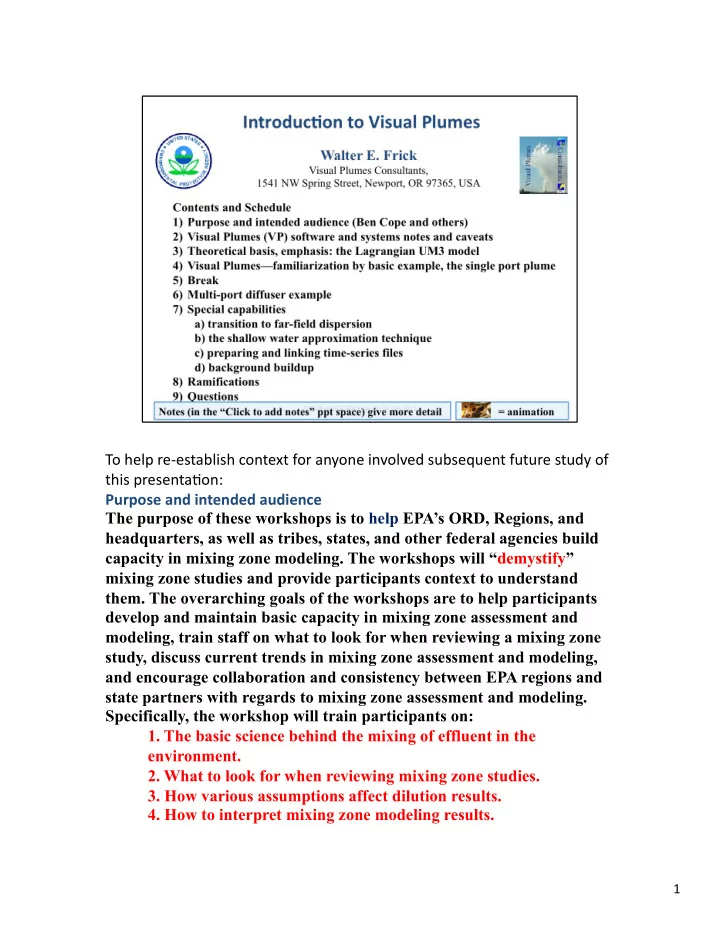
To ¡help ¡re-­‑establish ¡context ¡for ¡anyone ¡involved ¡subsequent ¡future ¡study ¡of ¡ this ¡presenta8on: ¡ Purpose ¡and ¡intended ¡audience ¡ The purpose of these workshops is to help EPA’s ORD, Regions, and headquarters, as well as tribes, states, and other federal agencies build capacity in mixing zone modeling. The workshops will “demystify” mixing zone studies and provide participants context to understand

• them. The overarching goals of the workshops are to help participants

develop and maintain basic capacity in mixing zone assessment and modeling, train staff on what to look for when reviewing a mixing zone study, discuss current trends in mixing zone assessment and modeling, and encourage collaboration and consistency between EPA regions and state partners with regards to mixing zone assessment and modeling. Specifically, the workshop will train participants on:

• 1. The basic science behind the mixing of effluent in the

environment.

• 2. What to look for when reviewing mixing zone studies.
• 3. How various assumptions affect dilution results.
• 4. How to interpret mixing zone modeling results.

1 ¡

2 ¡

3 ¡

4 ¡

Visual Plumes was developed in Windows XP and earlier versions of Microsoft Windows Operating System (OS). Beginning with Windows Vista it became difficult to compile VP (convert the computer code into executable language) VP. At this time VP is compiled on a Windows 7 machine through a Windows XP emulator. The computer language is Delphi 7 (a superset of Pascal) . VP uses the Borland Database Engine (BDE), software that supports the handling of the diffuser and ambient tables used in VP. Various other software applications also use the BDE engine. If the BDE engine is installed on any given computer (due to other prior application installations) then VP works directly after installing VP. If not, it is necessary to find a application which will install the BDE components. One such application is called BDEinfosetup.exe. While VPC owns the file, it is not clear that VPC can legally distribute it. Therefore, VPC depends on the user to acquire the necessary software. It may be possible that EPA could bundled the application with VP on the CEAM website. Users should also be aware that there are a few known bugs in VP that have not been fully identified and corrected. In some instances these are initialization problems that can be overcome by repeating the action again. In any case, the user is invited to report bugs so that future versions of VP may be corrected. VPC seeks to maintain VP in the public domain and offers to update older versions of VP for inclusion as updates on the EPA CEAM website. 5 ¡

This ¡slide ¡is ¡intended ¡as ¡a ¡reference ¡for ¡future ¡study ¡ 6 ¡

7 ¡

8 ¡

9 ¡

10 ¡

11 ¡

12 ¡

13 ¡

Models ¡such ¡as ¡DKHw ¡are ¡external ¡executable ¡files ¡(exe). ¡VP ¡sets ¡up ¡their ¡input ¡files, ¡calls ¡the ¡exe, ¡waits ¡for ¡ the ¡exe ¡to ¡finish, ¡then ¡looks ¡for ¡the ¡output ¡file, ¡reads ¡it, ¡and ¡interprets ¡the ¡informa8on ¡on ¡the ¡text ¡and ¡ graphics ¡tabs. ¡Problems ¡can ¡arise ¡when ¡the ¡exe ¡terminates ¡abnormally. ¡A ¡file ¡handling ¡problem ¡can ¡arise ¡ when ¡VP ¡then ¡reads ¡an ¡older ¡output ¡file, ¡which ¡is ¡not ¡always ¡apparent ¡when ¡several ¡consecu8ve ¡cases ¡are ¡

• involved. ¡

UM3 ¡is ¡a ¡na8ve ¡model ¡so ¡called ¡because ¡it ¡is ¡coded ¡into ¡the ¡VP ¡code. ¡This ¡makes ¡for ¡easier ¡control ¡for ¡the ¡ developer ¡as ¡model ¡and ¡interface ¡are ¡compiled ¡together. ¡ DKHw, ¡NRFIELD, ¡and ¡UM3 ¡are ¡ini8al ¡dilu8on ¡models ¡that ¡can ¡be ¡linked ¡with ¡the ¡Brooks ¡far-­‑field ¡model. ¡ What ¡is ¡in ¡the ¡names: ¡ DKHW: Physics-based exe, Eulerian numerical formulation, integral flux model. One or multi-port diffusers. Acronyms: Davis, Kannberg, Hirst model (w = Windows; Windows VP package). Previous versions DKHDEN, UDKHDEN (1985)…. Later compilations up to 2011…. NRFIELD: Empirical, dimensional analysis and curves fit to data; exe. Based on T-risers, for 4 or more ports. RSB in DOS Plumes, native, Roberts, Snyder, Baumgartner model. Roberts continues work on NRFIELD currently conducting experiments with dense discharges. UM3: Physics-based native, Lagrangian numerical formulation, material element model. One or multi-port

• diffusers. Merge (pre 1985), UMERGE (1985), UM (1993), UM3, Updated Merge 3-D model.

PDS: Eulerian integral flux surface plume model; exe. Buoyant discharges. Acronym: Prych, Davis, Shirazi model. DOS Plumes: predecessor of Visual Plumes, runs RSB (pre-NRFIELD) and UM (Updated Merge model; pre-UM3). Features auto cell-fill: displays similarity parameters, length scales, cormix classes. Dreamware prototype depicts wire-mesh graphics, like UM3, vector based. Brooks far-field algorithm is a set of equations for estimating dispersion (dilution) in the far-field, beyond the initial dilution phase of plume development.

14 ¡

15 ¡

16 ¡

17 ¡

Even at its simplest, plume modeling guidance can appear mysterious and

• ambiguous. Understanding the capabilities and limitations of available models can

help avoid pitfalls and confusion and promote confidence in model outputs. This section seeks to help the user demystify the art and science of plume modeling for themselves. 18 ¡

19 ¡

20 ¡

21 ¡ This ¡work ¡concerned ¡events ¡surrounding ¡Hurricane ¡Katrina, ¡2005. ¡ ¡ Note ¡the ¡Mississippi ¡River ¡flow ¡at ¡Baton ¡Rouge, ¡6000 ¡cubic ¡meters ¡per ¡second ¡equals ¡ about ¡212,000cfs. ¡This ¡is ¡about ¡3 ¡8mes ¡larger ¡than ¡the ¡8dal ¡Yaquina ¡River, ¡Oregon, ¡ however, ¡the ¡Mississippi ¡has ¡mul8ple ¡mouths, ¡including ¡the ¡Atchafalaya ¡River ¡that ¡ discharges ¡near ¡Morgan ¡City, ¡west ¡of ¡New ¡Orleans ¡(not ¡shown ¡here). ¡(This ¡note ¡refers ¡to ¡ another ¡comparisons ¡including ¡use ¡of ¡the ¡Visual ¡Plumes ¡PDS ¡river ¡discharge ¡model.) ¡

22 ¡ Another ¡output ¡of ¡the ¡modeling. ¡Note ¡the ¡intense ¡parts ¡of ¡the ¡plumes ¡penetrate ¡about ¡ 5km ¡into ¡the ¡Gulf. ¡

23 ¡ The ¡intense ¡parts ¡of ¡the ¡plumes ¡penetrate ¡about ¡5km ¡into ¡the ¡Gulf. ¡

24 ¡

Empirical ¡models ¡are ¡based ¡on ¡laboratory ¡measurements. ¡Lab ¡results ¡may ¡be ¡ficed ¡to ¡ model ¡parameters ¡that ¡are ¡derived ¡through ¡dimensional ¡analysis ¡or ¡other ¡techniques. ¡ Coefficients ¡are ¡established ¡that ¡produce ¡the ¡best ¡fits ¡and ¡similarity ¡theory ¡may ¡be ¡used ¡ to ¡generalize ¡the ¡results, ¡making ¡it ¡possible ¡to ¡adapt ¡results ¡to ¡larger ¡or ¡smaller ¡length ¡

• scales. ¡Similarity ¡may ¡be ¡achieved ¡by ¡matching ¡Froude ¡number, ¡stra8fica8on ¡number, ¡

Reynolds ¡number ¡and ¡other ¡similarity ¡parameters ¡or ¡length ¡scales. ¡Non-­‑linear ¡effects ¡like ¡ the ¡density ¡of ¡water ¡near ¡freezing ¡temperature ¡can ¡complicate ¡similarity ¡theory, ¡ some8mes ¡with ¡unexpected ¡and ¡significant ¡consequences. ¡ 25 ¡

26 ¡

27 ¡

Corjet, ¡one ¡of ¡the ¡models ¡in ¡Cormix, ¡ ¡is ¡also ¡an ¡Eulerian ¡integral ¡flux ¡model. ¡ DKH ¡refers ¡to ¡Davis, ¡Kannberg, ¡and ¡Hirst, ¡the ¡original ¡authors ¡of ¡DKHden ¡even ¡before ¡the ¡ UDKHDEN ¡and ¡UMERGE ¡(now ¡UM3) ¡models ¡were ¡published ¡in ¡the ¡EPA ¡publica8on ¡of ¡ EPA/600/3-­‑85/073a ¡and ¡b: ¡ ¡“Ini8al ¡mixing ¡characteris8cs ¡of ¡municipal ¡ocean ¡discharges” ¡ in ¡1985. ¡(Muellenhoff, ¡Soldate, ¡Baumgartner, ¡Schuldt, ¡Davis, ¡and ¡Frick.) ¡The ¡U ¡stood ¡for ¡ Universal ¡because ¡each ¡included ¡model ¡used ¡the ¡same ¡input ¡format ¡called ¡Universal ¡ Data ¡Files ¡(UDF) ¡files. ¡UM3 ¡now ¡might ¡suggest ¡the ¡“Updated ¡Merge ¡3-­‑dimensional” ¡

• model. ¡UMERGE ¡was ¡a ¡quasi ¡3-­‑D ¡model ¡whereas ¡UM3 ¡is ¡fully ¡three-­‑dimensional ¡when ¡

modeling ¡individual ¡plumes, ¡making ¡full ¡use ¡of ¡vector ¡algebra ¡to ¡represent ¡three-­‑ dimensional ¡physics. ¡ Cautionary DKHw and UDKHDEN notes for the record: 1) they do not report when the plumes intersect the receiving water surface 2) they hold plume spacing constant even when the current is not perpendicular to the diffuser axis (to be conservative the user should input the reduced spacing, the spacing distance projected to the current) 28 ¡

This ¡presenta8on ¡covers ¡a ¡lot ¡of ¡ground. ¡For ¡the ¡sake ¡of ¡8me ¡some ¡aspects ¡of ¡modeling ¡ are ¡emphasized ¡at ¡the ¡expense ¡of ¡other ¡aspects. ¡The ¡previous ¡Eulerian ¡model ¡ simula8ons ¡are ¡based ¡on ¡the ¡concept ¡of ¡steady ¡state. ¡This ¡means ¡that ¡the ¡predic8ons ¡ represent ¡8me-­‑averaged ¡behavior. ¡We ¡may ¡think ¡of ¡averaging ¡together ¡many ¡snapshots ¡

• f ¡the ¡instantaneous ¡plumes ¡that ¡are ¡quite ¡turbulent ¡and ¡heterogeneous. ¡The ¡result ¡of ¡

this ¡averaging ¡is ¡to ¡produce ¡smooth ¡surfaces ¡and ¡concentra8on ¡pacerns ¡as ¡shown ¡in ¡the ¡ upper ¡right ¡panel. ¡It ¡is ¡such ¡pacerns ¡and ¡concentra8ons ¡we ¡acempt ¡to ¡simulate. ¡To ¡ make ¡the ¡problem ¡tractable ¡we ¡assume ¡the ¡cross-­‑sec8on ¡is ¡round ¡but ¡already ¡recognize ¡ that ¡this ¡is ¡a ¡simplifica8on ¡which ¡can ¡have ¡significant ¡consequences. ¡In ¡current ¡the ¡ plumes ¡are ¡oken ¡kidney ¡shaped ¡as ¡shown ¡in ¡the ¡lower ¡right ¡panel. ¡If ¡stra8fica8on ¡is ¡ strong ¡the ¡cross-­‑sec8on ¡can ¡become ¡even ¡more ¡flacened ¡in ¡shape. ¡This ¡can ¡affect ¡our ¡ interpreta8on ¡of ¡when ¡the ¡plume’s ¡upper ¡surface ¡intersects ¡the ¡water ¡surface. ¡ 29 ¡

30 ¡

This ¡simula8on ¡is ¡not ¡based ¡on ¡actual ¡input ¡condi8ons, ¡which ¡are ¡unknown. ¡This ¡is ¡a ¡ crude ¡example ¡of ¡similarity. ¡The ¡actual ¡medium ¡is ¡air, ¡the ¡model ¡medium ¡is ¡water. ¡Input ¡ condi8ons ¡were ¡varied ¡un8l ¡a ¡fit, ¡rela8ve ¡to ¡a ¡common ¡diameter, ¡was ¡obtained. ¡Output ¡ was ¡set ¡up ¡to ¡plot ¡diameters ¡(denoted ¡by ¡red ¡dots) ¡and ¡at ¡constant ¡intervals ¡to ¡help ¡ represent ¡the ¡concept ¡of ¡control ¡volumes. ¡ Shown ¡is ¡a ¡UM3 ¡simula8on. ¡UM3 ¡was ¡modified ¡to ¡output ¡plume ¡diameters ¡(diameter ¡ endpoints) ¡whenever ¡the ¡travel ¡distance ¡increased ¡by ¡more ¡than ¡the ¡criterion ¡distance ¡ aker ¡the ¡previous ¡diameter ¡output. ¡The ¡apparent ¡lengthsds ¡of ¡the ¡control ¡volumes, ¡ which ¡should ¡be ¡equal, ¡differ ¡slightly ¡from ¡one ¡control ¡volume ¡to ¡the ¡next ¡because ¡the ¡ integra8on ¡step ¡is ¡variable ¡and ¡finite ¡(though ¡small). ¡ ¡As ¡several ¡steps ¡of ¡variable ¡size ¡are ¡ involved ¡between ¡outputs, ¡the ¡accumulated ¡distance ¡varies ¡from ¡one ¡cross-­‑sec8on ¡to ¡ the ¡next. ¡ The ¡control ¡volume ¡length ¡could ¡be ¡varied ¡as ¡part ¡of ¡a ¡model ¡convergence ¡scheme ¡but ¡ the ¡main ¡idea ¡is ¡that ¡the ¡volumes ¡are ¡sta8onary ¡with ¡mass ¡flux ¡in ¡(from ¡the ¡source, ¡from ¡ the ¡upstream ¡control ¡volume, ¡or ¡from ¡the ¡surroundings) ¡or ¡out ¡(to ¡enter ¡the ¡ downstream ¡control ¡volume). ¡ 31 ¡

32 ¡

The ¡DOS ¡Plumes ¡manual ¡covers ¡the ¡Lagrangian ¡theory ¡in ¡some ¡detail. ¡The ¡first ¡journal ¡ ar8cle ¡to ¡outline ¡the ¡complete ¡plume ¡theory ¡(excluding ¡merging ¡and ¡other ¡out ¡of ¡scope ¡ complica8ons) ¡was ¡published ¡in ¡1984. ¡The ¡finite-­‑difference ¡model, ¡which ¡is ¡very ¡useful ¡ for ¡understanding ¡the ¡prac8cali8es ¡of ¡numerical ¡modeling ¡of ¡this ¡type, ¡is ¡found ¡in ¡ EPA-­‑600/3-­‑76-­‑100 ¡(Cooling ¡tower ¡plume ¡model), ¡1976. ¡ 33 ¡

Presumably ¡no ¡Eulerian ¡modeler ¡has ¡to ¡prove ¡equivalence ¡with ¡the ¡Lagrangian ¡ formula8on ¡ ¡ 34 ¡

Actually, ¡a ¡more ¡useful ¡analogy ¡to ¡plumes ¡would ¡be ¡two ¡cars ¡possessing ¡the ¡same ¡speed ¡ as ¡they ¡pass ¡through ¡the ¡light ¡but ¡car ¡2 ¡passing ¡that ¡point ¡one ¡second ¡behind ¡car ¡1. ¡If ¡ they ¡prac8ce ¡the ¡same ¡driving ¡pacern ¡(steady ¡state) ¡their ¡distance ¡apart ¡will ¡either ¡ increase ¡or ¡decrease ¡depending ¡on ¡whether ¡they ¡speed ¡up ¡or ¡slow ¡down ¡down ¡the ¡road. ¡ Now ¡you ¡know ¡why ¡trucks ¡are ¡usually ¡closer ¡together ¡on ¡steep ¡grades. ¡They ¡may ¡be ¡ spacing ¡themselves, ¡say, ¡2 ¡seconds ¡apart. ¡ 35 ¡

In ¡Lagrangian ¡theory ¡all ¡the ¡material ¡in ¡the ¡plume ¡element ¡at ¡its ¡incep8on ¡remain ¡in ¡the ¡ plume ¡element. ¡In ¡this ¡sense ¡it ¡is ¡a ¡material ¡element. ¡Its ¡increase ¡in ¡volume ¡is ¡due ¡to ¡ entrainment ¡plus ¡changes ¡in ¡density ¡that ¡come ¡about ¡from ¡water’s ¡density ¡non-­‑linear ¡ response ¡to ¡salinity ¡and ¡temperature. ¡ As ¡the ¡leading ¡and ¡trailing ¡faces ¡occupy ¡posi8on ¡a ¡given ¡amount ¡of ¡8me ¡different ¡in ¡age, ¡ h ¡= ¡(instantaneous ¡speed)(t2-­‑t1). ¡Given ¡steady ¡state, ¡the ¡height ¡h ¡is ¡a ¡only ¡a ¡func8on ¡of ¡ the ¡instantaneous ¡speed ¡because ¡t2-­‑t1) ¡is ¡constant ¡while ¡steady ¡state ¡is ¡maintained. ¡ ¡ Actual ¡plume ¡elements ¡are ¡shorter, ¡exaggerated ¡here ¡for ¡instruc8onal ¡purposes. ¡In ¡ ini8alizing ¡condi8ons ¡UM3 ¡sets ¡h(0) ¡to ¡one-­‑tenth ¡of ¡the ¡ini8al ¡diameter. ¡The ¡ini8al ¡8me ¡ step ¡(Δt)o ¡is ¡correspondingly ¡small. ¡ 36 ¡

This ¡effect ¡is ¡some8mes ¡referred ¡to ¡as ¡the ¡“jelly ¡sandwich” ¡equa8on. ¡Squeeze ¡both ¡ends ¡ and ¡the ¡diameter ¡increases. ¡Pull ¡both ¡ends ¡outward, ¡like ¡bellows, ¡and ¡the ¡diameter ¡

• decreases. ¡This ¡is ¡in ¡the ¡absence ¡of ¡entrainment, ¡which ¡may ¡mask ¡some ¡of ¡the ¡jelly-­‑

sandwich ¡effect. ¡ 37 ¡

38 ¡

39 ¡

40 ¡

41 ¡

42 ¡

Understanding the significance of the steady state assumption ultimately lead to a completely new conception of the plume element. The right-cylinder tuna can was replaced by a section from a bent cone. The trick became to accurately derive the projected area of the plume element’s surface as a function of r, h, and θ, the trajectory inclination angle to the horizontal axis. First assuming that the plume element height (h) was constant (the “tuna can,” right cylinder conception of the Lagrangian plume element) Winiarski and Frick formulated about 20 different entrainment functions, some leading to fabulous, but wrong, solutions, like blowing up. After suspecting that perhaps h could not be assumed constant, W&F rather quickly formulated the current expression for forced entrainment, probably less than 5. First, an examination of Fan’s dilution and radii data confirmed that they were not directly proportional or linearly related. Something like the car analogy, followed by the rigorous integration found in the DOS Plumes manual, was then used to develop the “free” equation for h. UM3 equations are based on the “top hat” assumption, that plume properties are average values when it comes to expressing the equations of motion. This is an idealization,

• bviously plume centerline properties are different from edge properties. In omitting a

pressure force on the plume, they reasoned that plume properties “feathered” into ambient properties at the plume’s edge, hence no pressure force as would be experienced by a solid object. 43 ¡

44 ¡ Dream ¡model ¡consider ¡mass ¡distribu8on ¡about ¡the ¡center ¡of ¡mass ¡(not ¡the ¡center ¡of ¡the ¡ cross ¡sec8on). ¡Overlap ¡is ¡dealt ¡with ¡explicitly. ¡ Schema8c ¡diagrams ¡illustra8ng ¡details ¡of ¡plume ¡merging ¡theory; ¡the ¡plume ¡element ¡as ¡a ¡ wedge-­‑shaped, ¡overlapped ¡en8ty; ¡mass ¡about ¡to ¡collide ¡with ¡the ¡plume ¡to ¡become ¡ entrained ¡mass—part ¡of ¡the ¡plume. ¡

Differential equations (DE) express changes with time or distance Usually the changes are smooth and continuous The plume DE can not be solved analytically The DE must be solved numerically: a finite difference approach For the Lagrangian model the infinitesimal integrating factor like dt is replaced by Δt: t2 – t1 For the Eulerian integral flux the infinitesimal integrating factor ds is replaced by Δs: s2 – s1 The numeric integration is stepwise If Δt or Δs are too large the solution diverges from the true solution because the Δt or Δs too crude to capture rapid changes If Δt or Δs are too small the solution diverges from truncation errors The plume equations are sometimes called stiff: at first Δt or Δs must be tiny but if constant truncation errors build up Convergence schemes are needed, for example, dt must increase as the plume solution develops Good increase schemes for Δt or Δs yield solutions that converge Crude schemes cause divergence or quantum jumps, i.e., a tiny change in current angle will cause a not insignificant change in dilution prediction simply because the integrating factor adjustment was too coarse. UM3 is very continuous ¡ 45 ¡

46 ¡

47 ¡

48 ¡

49 ¡

50 ¡

51 ¡

52 ¡

53 ¡

54 ¡

55 ¡

side ¡view ¡ ¡ ¡0.0001 ¡ ¡ ¡1.0145 ¡ ¡ ¡0.0068 ¡ ¡ ¡1.0157 ¡ ¡ ¡0.0149 ¡ ¡ ¡1.0158 ¡ ¡ ¡0.0197 ¡ ¡ ¡1.0161 ¡ ¡ ¡0.0264 ¡ ¡ ¡1.0159 ¡ ¡ ¡0.0339 ¡ ¡ ¡1.0164 ¡ ¡ ¡0.0423 ¡ ¡ ¡1.0182 ¡ ¡ ¡0.0491 ¡ ¡ ¡1.0191 ¡ ¡ ¡0.0565 ¡ ¡ ¡1.0180 ¡ ¡ ¡0.0638 ¡ ¡ ¡1.0180 ¡ ¡ ¡0.0676 ¡ ¡ ¡1.0186 ¡ ¡ ¡0.0776 ¡ ¡ ¡1.0177 ¡ ¡ ¡0.0830 ¡ ¡ ¡1.0169 ¡ ¡ ¡0.0912 ¡ ¡ ¡1.0146 ¡ ¡ ¡0.1000 ¡ ¡ ¡1.0118 ¡ ¡ ¡0.1084 ¡ ¡ ¡1.0100 ¡ ¡ ¡0.1155 ¡ ¡ ¡1.0053 ¡ ¡ ¡0.1181 ¡ ¡ ¡1.0024 ¡ ¡ ¡0.1236 ¡ ¡ ¡1.0003 ¡ ¡ ¡0.1285 ¡ ¡ ¡0.9976 ¡ ¡ ¡0.1336 ¡ ¡ ¡0.9924 ¡ ¡ ¡0.1391 ¡ ¡ ¡0.9854 ¡ ¡ ¡0.1420 ¡ ¡ ¡0.9819 ¡ ¡ ¡0.1482 ¡ ¡ ¡0.9789 ¡ ¡ ¡0.1543 ¡ ¡ ¡0.9758 ¡ ¡ ¡0.1585 ¡ ¡ ¡0.9709 ¡ ¡ ¡0.1642 ¡ ¡ ¡0.9662 ¡ ¡ ¡0.1709 ¡ ¡ ¡0.9600 ¡ ¡ ¡0.1773 ¡ ¡ ¡0.9530 ¡ ¡ ¡0.1835 ¡ ¡ ¡0.9500 ¡ ¡ ¡0.1889 ¡ ¡ ¡0.9468 ¡ ¡ ¡0.1950 ¡ ¡ ¡0.9400 ¡ ¡ ¡0.1999 ¡ ¡ ¡0.9343 ¡ ¡ ¡0.2023 ¡ ¡ ¡0.9303 ¡ ¡ ¡0.2092 ¡ ¡ ¡0.9261 ¡ ¡ ¡0.2168 ¡ ¡ ¡0.9239 ¡ ¡ ¡0.2253 ¡ ¡ ¡0.9205 ¡ ¡ ¡0.2327 ¡ ¡ ¡0.9173 ¡ ¡ ¡0.2385 ¡ ¡ ¡0.9114 ¡ ¡ ¡0.2422 ¡ ¡ ¡0.9049 ¡ ¡ ¡0.2431 ¡ ¡ ¡0.9019 ¡ ¡ ¡0.2478 ¡ ¡ ¡0.8989 ¡ ¡ ¡0.2504 ¡ ¡ ¡0.8942 ¡ ¡ ¡0.2550 ¡ ¡ ¡0.8907 ¡ ¡ ¡0.2615 ¡ ¡ ¡0.8878 ¡ ¡ ¡0.2684 ¡ ¡ ¡0.8849 ¡ ¡ ¡0.2777 ¡ ¡ ¡0.8826 ¡ ¡ ¡0.2865 ¡ ¡ ¡0.8804 ¡ ¡ ¡0.2968 ¡ ¡ ¡0.8786 ¡ ¡ ¡0.3072 ¡ ¡ ¡0.8770 ¡ ¡ ¡0.3134 ¡ ¡ ¡0.8768 ¡ ¡ ¡0.3239 ¡ ¡ ¡0.8781 ¡ ¡ ¡0.3308 ¡ ¡ ¡0.8799 ¡ ¡ ¡0.3395 ¡ ¡ ¡0.8789 ¡ ¡ ¡0.3428 ¡ ¡ ¡0.8777 ¡ ¡ ¡0.3528 ¡ ¡ ¡0.8789 ¡ ¡ ¡0.3616 ¡ ¡ ¡0.8796 ¡ ¡ ¡0.3701 ¡ ¡ ¡0.8795 ¡ ¡ ¡0.3777 ¡ ¡ ¡0.8792 ¡ ¡ ¡0.3876 ¡ ¡ ¡0.8796 ¡ ¡ ¡0.3947 ¡ ¡ ¡0.8796 ¡ ¡ ¡0.4032 ¡ ¡ ¡0.8812 ¡ ¡ ¡0.4095 ¡ ¡ ¡0.8827 ¡ ¡ ¡0.4193 ¡ ¡ ¡0.8832 ¡ ¡ ¡0.4288 ¡ ¡ ¡0.8831 ¡ ¡ ¡0.4373 ¡ ¡ ¡0.8854 ¡ ¡ ¡0.4468 ¡ ¡ ¡0.8878 ¡ ¡ ¡0.4047 ¡ ¡ ¡0.7966 ¡ ¡ ¡0.3985 ¡ ¡ ¡0.7965 ¡ ¡ ¡0.3920 ¡ ¡ ¡0.7966 ¡ ¡ ¡0.3855 ¡ ¡ ¡0.7961 ¡ ¡ ¡0.3800 ¡ ¡ ¡0.7961 ¡ ¡ ¡0.3723 ¡ ¡ ¡0.7958 ¡ ¡ ¡0.3651 ¡ ¡ ¡0.7943 ¡ ¡ ¡0.3581 ¡ ¡ ¡0.7932 ¡ ¡ ¡0.3536 ¡ ¡ ¡0.7918 ¡ ¡ ¡0.3477 ¡ ¡ ¡0.7923 ¡ ¡ ¡0.3420 ¡ ¡ ¡0.7927 ¡ ¡ ¡0.3353 ¡ ¡ ¡0.7920 ¡ ¡ ¡0.3286 ¡ ¡ ¡0.7884 ¡ ¡ ¡0.3254 ¡ ¡ ¡0.7864 ¡ ¡ ¡0.3211 ¡ ¡ ¡0.7843 ¡ ¡ ¡0.3169 ¡ ¡ ¡0.7831 ¡ ¡ ¡0.3116 ¡ ¡ ¡0.7834 ¡ ¡ ¡0.3077 ¡ ¡ ¡0.7838 ¡ ¡ ¡0.3027 ¡ ¡ ¡0.7849 ¡ ¡ ¡0.2977 ¡ ¡ ¡0.7858 ¡ ¡ ¡0.2934 ¡ ¡ ¡0.7868 ¡ ¡ ¡0.2899 ¡ ¡ ¡0.7850 ¡ ¡ ¡0.2864 ¡ ¡ ¡0.7830 ¡ ¡ ¡0.2838 ¡ ¡ ¡0.7826 ¡ ¡ ¡0.2791 ¡ ¡ ¡0.7826 ¡ ¡ ¡0.2762 ¡ ¡ ¡0.7826 ¡ ¡ ¡0.2739 ¡ ¡ ¡0.7804 ¡ ¡ ¡0.2674 ¡ ¡ ¡0.7762 ¡ ¡ ¡0.2626 ¡ ¡ ¡0.7728 ¡ ¡ ¡0.2568 ¡ ¡ ¡0.7707 ¡ ¡ ¡0.2507 ¡ ¡ ¡0.7673 ¡ ¡ ¡0.2435 ¡ ¡ ¡0.7646 ¡ ¡ ¡0.2351 ¡ ¡ ¡0.7643 ¡ ¡ ¡0.2262 ¡ ¡ ¡0.7635 ¡ ¡ ¡0.2165 ¡ ¡ ¡0.7647 ¡ ¡ ¡0.2086 ¡ ¡ ¡0.7668 ¡ ¡ ¡0.2035 ¡ ¡ ¡0.7691 ¡ ¡ ¡0.1999 ¡ ¡ ¡0.7749 ¡ ¡ ¡0.1945 ¡ ¡ ¡0.7786 ¡ ¡ ¡0.1870 ¡ ¡ ¡0.7816 ¡ ¡ ¡0.1800 ¡ ¡ ¡0.7843 ¡ ¡ ¡0.1714 ¡ ¡ ¡0.7882 ¡ ¡ ¡0.1659 ¡ ¡ ¡0.7926 ¡ ¡ ¡0.1586 ¡ ¡ ¡0.7973 ¡ ¡ ¡0.1519 ¡ ¡ ¡0.8016 ¡ ¡ ¡0.1441 ¡ ¡ ¡0.8049 ¡ ¡ ¡0.1376 ¡ ¡ ¡0.8078 ¡ ¡ ¡0.1293 ¡ ¡ ¡0.8107 ¡ ¡ ¡0.1184 ¡ ¡ ¡0.8134 ¡ ¡ ¡0.1097 ¡ ¡ ¡0.8153 ¡ ¡ ¡0.1020 ¡ ¡ ¡0.8166 ¡ ¡ ¡0.0942 ¡ ¡ ¡0.8172 ¡ ¡ ¡0.0847 ¡ ¡ ¡0.8176 ¡ ¡ ¡0.0769 ¡ ¡ ¡0.8193 ¡ ¡ ¡0.0672 ¡ ¡ ¡0.8201 ¡ ¡ ¡0.0595 ¡ ¡ ¡0.8228 ¡ ¡ ¡0.0514 ¡ ¡ ¡0.8216 ¡ ¡ ¡0.0457 ¡ ¡ ¡0.8208 ¡ ¡ ¡0.0408 ¡ ¡ ¡0.8236 ¡ ¡ ¡0.0338 ¡ ¡ ¡0.8266 ¡ ¡ ¡0.0291 ¡ ¡ ¡0.8284 ¡ ¡ ¡0.0199 ¡ ¡ ¡0.8291 ¡

56 ¡

0.0170 ¡ ¡ ¡0.8577 ¡ ¡ ¡0.0212 ¡ ¡ ¡0.8574 ¡ ¡ ¡0.0278 ¡ ¡ ¡0.8569 ¡ ¡ ¡0.0358 ¡ ¡ ¡0.8608 ¡ ¡ ¡0.0459 ¡ ¡ ¡0.8615 ¡ ¡ ¡0.0530 ¡ ¡ ¡0.8605 ¡ ¡ ¡0.0630 ¡ ¡ ¡0.8591 ¡ ¡ ¡0.0726 ¡ ¡ ¡0.8601 ¡ ¡ ¡0.0808 ¡ ¡ ¡0.8641 ¡ ¡ ¡0.0884 ¡ ¡ ¡0.8705 ¡ ¡ ¡0.0953 ¡ ¡ ¡0.8736 ¡ ¡ ¡0.1012 ¡ ¡ ¡0.8759 ¡ ¡ ¡0.1061 ¡ ¡ ¡0.8820 ¡ ¡ ¡0.1100 ¡ ¡ ¡0.8908 ¡ ¡ ¡0.1105 ¡ ¡ ¡0.8977 ¡ ¡ ¡0.1100 ¡ ¡ ¡0.9073 ¡ ¡ ¡0.1101 ¡ ¡ ¡0.9118 ¡ ¡ ¡0.1111 ¡ ¡ ¡0.9166 ¡ ¡ ¡0.1123 ¡ ¡ ¡0.9216 ¡ ¡ ¡0.1124 ¡ ¡ ¡0.9236 ¡ ¡ ¡0.1100 ¡ ¡ ¡0.9304 ¡ ¡ ¡0.1073 ¡ ¡ ¡0.9380 ¡ ¡ ¡0.1026 ¡ ¡ ¡0.9464 ¡ ¡ ¡0.0997 ¡ ¡ ¡0.9524 ¡ ¡ ¡0.0962 ¡ ¡ ¡0.9597 ¡ ¡ ¡0.0924 ¡ ¡ ¡0.9673 ¡ ¡ ¡0.0839 ¡ ¡ ¡0.9769 ¡ ¡ ¡0.0777 ¡ ¡ ¡0.9828 ¡ ¡ ¡0.0693 ¡ ¡ ¡0.9870 ¡ ¡ ¡0.0624 ¡ ¡ ¡0.9920 ¡ ¡ ¡0.0541 ¡ ¡ ¡0.9959 ¡ ¡ ¡0.0485 ¡ ¡ ¡0.9988 ¡ ¡ ¡0.0411 ¡ ¡ ¡1.0011 ¡ ¡ ¡0.0343 ¡ ¡ ¡1.0028 ¡ ¡ ¡0.0273 ¡ ¡ ¡1.0065 ¡ ¡ ¡0.0212 ¡ ¡ ¡1.0084 ¡ ¡ ¡0.0168 ¡ ¡ ¡1.0095 ¡ ¡ ¡0.0099 ¡ ¡ ¡1.0114 ¡ ¡ ¡0.0042 ¡ ¡ ¡1.0126 ¡ ¡-­‑0.0001 ¡ ¡ ¡1.0124 ¡ density ¡profile ¡ 17.3 ¡0.0 ¡ 25.2 ¡1.0 ¡

57 ¡

58 ¡

59 ¡

60 ¡

61 ¡

62 ¡

63 ¡

Work ¡done ¡by ¡Liseth ¡(reference ¡not ¡immediately ¡available) ¡shows ¡plumes ¡generate ¡ current ¡around ¡themselves. ¡Here ¡iden8cal ¡single ¡and ¡double ¡plumes ¡of ¡equal ¡ densimetric ¡Froude ¡are ¡shown ¡in ¡two ¡sets ¡of ¡experiments. ¡It ¡is ¡striking ¡how ¡in ¡pairs ¡the ¡ plumes ¡“acract” ¡each ¡other. ¡ 64 ¡

65 ¡

66 ¡

67 ¡

68 ¡

69 ¡

70 ¡

71 ¡

72 ¡