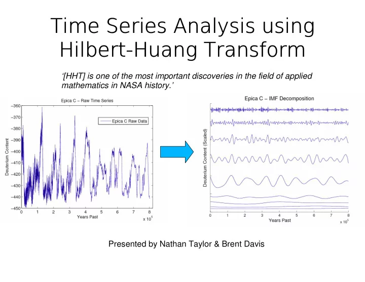
SLIDE 1 Time Series Analysis using Hilbert-Huang Transform
‘[HHT] is one of the most important discoveries in the field of applied mathematics in NASA history.’ Presented by Nathan Taylor & Brent Davis
SLIDE 2
SLIDE 3
Terminology
Hilbert-Huang Transform (HHT) Empirical Mode Decomposition (EMD) Ensemble Empirical Mode Decomposition (EEMD) Intrinsic Mode Function (IMF) Empirical – Relying on derived from observation or experiment Mode – A particular form, variety, or manner Decomposition – The separation of a whole into basic parts Intrinsic – Belonging naturally
SLIDE 4 Computing the high frequency IMF
Find all local maxima of TS Find all local minima of TS Fit a curve through maxima Fit a curve through minima Find the mean of these two curves
SLIDE 5
Sifting: Subtract mean from Original Time Series
Subtract the mean from original TS The goal is after a number of siftings, to minimize the mean
SLIDE 6
Repeat this process of sifting
Three Notes: The mean will approach zero. The two envelopes are becoming more symmetric.
SLIDE 7
After multiple siftings Q: What property does it have?
The mean is now minimized, so we would like to develop a stopping criterion a) b) The number of extrema and zero crossings are alternating.
SLIDE 8
EPICA C Ice Core IMF 1
The first IMF should have the highest frequency component.
SLIDE 9 Decomposing TS after multiple siftings
Residual + IMF1 = Original TS, Residual = Original TS – IMF1 . . .
Trend = Original TS – (IMF1 + IMF2 + … + IMFN)
SLIDE 10
SLIDE 11 About the trend
An application
a empirical trend line. The trend shouldn't have periodic behavior Here's the last IMF and original TS
SLIDE 12
SLIDE 13
SLIDE 14
SLIDE 15
SLIDE 16
SLIDE 17
SLIDE 18
SLIDE 19
SLIDE 20
What is mode mixing?
Cubic spline are not perfect if envelopes are close together and at a height away from zero Each IMF should have a dominant signal. Rather than get clean IMF signals there are combinations of frequencies
SLIDE 21 Explanation of EEMD
Ensemble - A unit or group of complementary parts that contribute to a single effect. Outline:
Add white noise to original TS Create a set of IMFs using EMD Do this N times Take the average of each individual IMF
Result: New set of IMFs with less mode mixing
SLIDE 22
EMD
SLIDE 23
EEMD with 500 iterations
SLIDE 24 Nonlinear Nonstationary (mean, variance
are functions of time
Local (frequency is
a function t)
Adaptive
FFT Frequency Power Spectrum: Mathematical artifacts
assume linear, stationary, global, and/or nonadaptive
SLIDE 25
Analysis of each IMF
SLIDE 26
SLIDE 27 Mathematical Artifacts of Time Series Analysis using HHT
Spacing:
- Even vs. Uneven
- Length of spacing
Curve Fitting:
- Cubic Spline vs. Linear Interpolation
Level of white noise added We'll use the Vostok & Epica C Ice Core Data for examples
SLIDE 28 Uneven versus Even Spacing – IMF 8
Notice the EEMD on the evenly spaced data pulls out a more uniform signal
SLIDE 29 EMD v. EEMD – Cubic Spline IMF 8
Notice the EEMD pulls out a more uniform signal
SLIDE 30 Linear Interpolation v. Cubic Spline – IMF 6
The cubic spline and the linear interpolation return almost the exact same signal
SLIDE 31 Choices in Length of Spacing – IMF 6
The difference in spacing has little effect on the signal pulled out.
SLIDE 32 Varying Levels of Noise
Notice the decompositions with higher levels of noise pull out a more uniform signal.
SLIDE 33 An Application of EEMD to Paleoclimatology
Paleoclimatology is the study
- f climate change on a long
time scale typically using a proxy measurement. We looked at two: EPICA C Ice Core Data Measures Deuterium Content
SLIDE 34
SLIDE 35
SLIDE 36
Noise of 0.5 Ensemble of 500 IMF 5 IMF 4 IMF 3
SLIDE 37 Welch Power Spectrum and Mean Periods of IMFs
Notice there are three noticeable peaks in each
100,000 year cycle? 40,000 year cycle? 20,000 year cycle?
SLIDE 38 Milankovitch cycles:
The earth axis completes one full cycle of precession every 26,000 years. The angle between Earth's rotational axis and the normal to the plane of its orbit, its obliquity, completes a full cycle every 41,000 years. The eccentricity is a measure of the departure of this ellipse from circularity Which combines to an approximate 100,000 year full cycle.
SLIDE 39 The angle between Earth's rotational axis and the normal to the plane of its orbit, its obliquity, completes a full cycle every 41,000 years.
SLIDE 40
SLIDE 41
Epica C Correlation Results for Obliquity & IMF 4
Lag results: 6,820 years ahead yields 0.6964 Choice: If the obliquity is a forcing function with which the earth responds, then the lag is 6,820 years ahead.
SLIDE 42 Correlation between IMF 4 and Obliquity
without lag: coefficient: 0.3444 significance: 0.6220 with lag: coefficient: 0.6954 significance: 1.0000
SLIDE 43 The eccentricity is a measure of the departure of this ellipse from circularity which combines to an approximate 100,000 year full cycle.
SLIDE 44 Correlation between IMF 5 and Eccentricity
coefficient: 0.5992 significance: 0.9940
SLIDE 45 The earth axis completes one full cycle of precession every 26,000 years.
SLIDE 46
SLIDE 47
SLIDE 48
Epica C Correlation Results for Climatic Precession & IMF 3
Lag results: 16,368 years ahead yields 0.4225 Choice: If the precession is a forcing function with which the earth responds, then the lag is 16,368 years ahead.
SLIDE 49
SLIDE 50
Correlation between IMF 3 and Climatic Precession
without lag: coefficient: -0.164 significance: 0.35 with lag: coefficient: 0.4225 significance: 0.9100