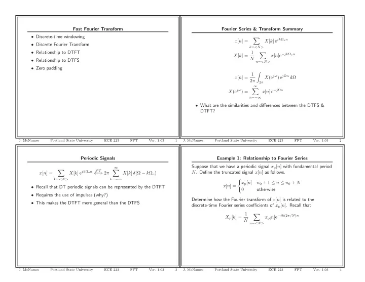
SLIDE 5 w = 0.0001:(2*pi)/1000:2*pi; X = (-exp(-j*w*1) + exp(-j*w*5) + exp(-j*w*13) - exp(-j*w*17))./(1-exp(-j*w)); % True spectrum figure FigureSet(1,’LTX’); subplot(2,1,1); h = plot(w,real(X),’r’,we,real(Xe),’k’); set(h(2),’Marker’,’o’); set(h(2),’MarkerFaceColor’,’k’); set(h(2),’MarkerSize’,3); ylabel(’Real X(e^{j\omega})’); xlim([0 pi]); box off; AxisLines; legend(h(1:2),’True DTFT’,’DFT Estimate’,4); subplot(2,1,2); h = plot(w,imag(X),’r’,we,imag(Xe),’k’); set(h(2),’Marker’,’o’); set(h(2),’MarkerFaceColor’,’k’); set(h(2),’MarkerSize’,3); ylabel(’Imag X(e^{j\omega})’); xlim([0 pi]); box off; AxisLines; xlabel(’Frequency (rads per sample)’); AxisSet(8); print -depsc FFTEstimate; %============================================================================== % Plot the True Transform \& Estimate %============================================================================== n = 1:16; x = -1*(n>=1 & n<=4) + 1*(n>=13 & n<=16); N = 2^(ceil(log2(2000))); k = 0:N-1; we = (0:N-1)*(2*pi/N); % Frequency of estimates Xe = exp(-j*k*(2*pi/N)*1).*fft(x,N);
Portland State University ECE 223 FFT
19
Example 3: DTFT Estimate with Padding
0.5 1 1.5 2 2.5 3 −10 −5 5 Real X(ejω) True DTFT DFT Estimate 0.5 1 1.5 2 2.5 3 −5 5 10 Imag X(ejω) Frequency (rads per sample)
Portland State University ECE 223 FFT
17
figure FigureSet(1,’LTX’); subplot(2,1,1); h = plot(w,real(X),’r’,we,real(Xe),’k’); set(h(1),’LineWidth’,2.0); set(h(2),’LineWidth’,1.0); ylabel(’Real X(e^{j\omega})’); xlim([0 pi]); box off; AxisLines; legend(h(1:2),’True DTFT’,’DFT Estimate’,4); subplot(2,1,2); h = plot(w,imag(X),’r’,we,imag(Xe),’k’); set(h(1),’LineWidth’,2.0); set(h(2),’LineWidth’,1.0); ylabel(’Imag X(e^{j\omega})’); xlim([0 pi]); box off; AxisLines; xlabel(’Frequency (rads per sample)’); AxisSet(8); print -depsc FFTEstimatePadded;
Portland State University ECE 223 FFT
20
Example 3: MATLAB Code
%function [] = FFTEstimate(); close all; n = 0:17; x = -1*(n>=1 & n<=4) + 1*(n>=13 & n<=16); %============================================================================== % Plot the signal %============================================================================== figure FigureSet(1,4.5,2.8); plot([min(n) max(n)],[0 0],’k:’); hold on; h = stem(n,x,’b’); set(h(1),’MarkerFaceColor’,’b’); set(h(1),’MarkerSize’,4); hold off; ylabel(’x[n]’); xlabel(’Time’); xlim([min(n) max(n)]); ylim([-1.05 1.05]); box off; AxisSet(8); print -depsc FFTESignal; %============================================================================== % Plot the True Transform \& Estimate %============================================================================== n = 1:16; x = -1*(n>=1 & n<=4) + 1*(n>=13 & n<=16); N = length(x); k = 0:N-1; we = (0:N-1)*(2*pi/N); % Frequency of estimates Xe = exp(-j*k*(2*pi/N)*1).*fft(x);
Portland State University ECE 223 FFT
18