This image from page 60 of your manual shows you what you should see - - PDF document

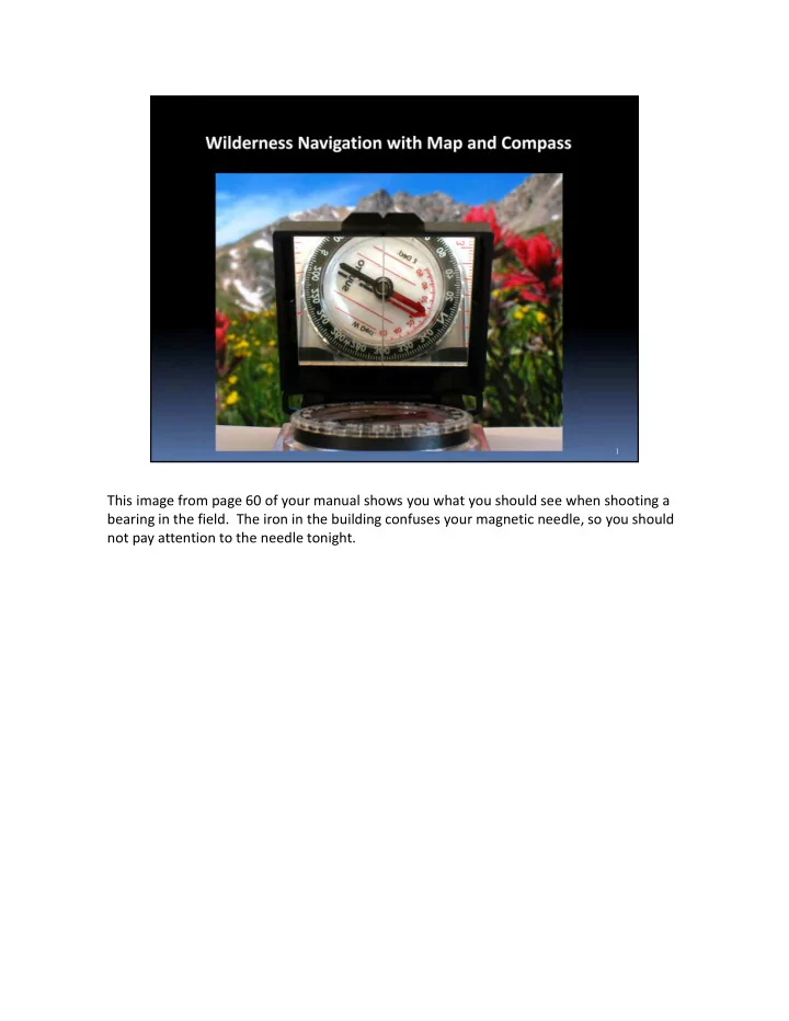
This image from page 60 of your manual shows you what you should see when shooting a bearing in the field. The iron in the building confuses your magnetic needle, so you should not pay attention to the needle tonight.

Our Map and Compass field day is a lot like an Easter egg hunt, but you will be looking for colored flagging tape rather than eggs. In addition, we give you a map and tell you where the points are, since we do not want you to wander around there aimlessly.

(Notes will be omitted on those pages where they are not necessary.)

Beginning on page xxvii you will find the descriptions of the points. If you’re new to this the descriptions may seem obscure and even intimidating. One of our goals is to make this statement useful to you. By learning how to interpret this statement you will master the techniques of a wilderness navigator.

There are three basic concepts that affect your journey to your destination: direction, distance, and topography. The brown ovals, called contour lines, schematically represent the topography. Imagine that they denote a mountain. Because of the topography a straight line is rarely the best route to your destination. Choosing your path is called route

• finding. The path you choose will depend on your goals for the hike. It is a sad fact of life

that all three concepts involve numbers. You are used to that for distance and topography, but we don’t usually associate a number with direction. We will cover that first.

In town the streets give us direction, so most people in Golden do not worry about the exact direction of north. In the wilderness we have no streets to guide us, so we must think more carefully about our direction of travel.

You are probably familiar with the cardinal directions (north, east, south, and west) and the

• rdinal directions (northeast, southeast, southwest, and northwest). This system of

naming has been pushed up to 32 directions with names like north by east, north‐ northeast, northeast by north, etc. It gets awkward, and we need more than 32 directions. We will instead use a simpler system in which we divide the circle into 360 directions and number them. The compass rose above gives you a hint of how it works.

We call these numbers degrees. If the name evokes traumatic memories of trigonometry class, you may relax. You do not need trig for this course. Memorize the number of degrees for each cardinal direction!

To help us get used to this system, we’re going to figure out what direction you are facing when sitting in the auditorium. For that we’ll use the kind of map you will be using in your wilderness navigation. North now points straight up. These maps do not use a compass rose, but the symbol just to the left of bottom shows the direction of north with the little star, which represents the north star. By the way, black is used to show buildings and surface streets. Gray is used to show urban areas. Major highways are shown in red. Blue is for water. The brown lines are the contours. We’ll discuss them later.

The rows of chairs in the auditorium are parallel to 10th St. Using my compass as a protractor, I measured the direction of 10th St. And Washington Ave. When you look straight ahead, you are facing in the direction we call 324 degrees.

To reverse a direction simply add or subtract 180 degrees. If mental arithmetic gives you a headache, do not worry. Your compass will do it for you.

Your compass dial uses the system I have just showed you. Because of the thickness of the marks, only the even‐numbered directions are shown. At the very top there is a clear arrow point lined up with 0 degrees. We call that the index mark. There is a similar mark

• n the opposite side at 180 degrees. If you turn the dial so that 54 degrees is at the index

mark, you can read off 234 degrees at the opposite mark.

This numbering system can also be used to describe our position on the Earth’s surface. If you need to summon a helicopter to your location, the pilot will want to know your latitude and longitude. Let’s review how it works. There are two sets of circles: parallels running east‐west, and meridians running north‐south. The intersection of a parallel with a meridian determines a point. The parallels show your latitude. For instance, every point

• n the circle N30º is 30 degrees north of the Equator. (Baseline Rd in Boulder is exactly 40º

N.) The meridians show your longitude. Every point on W50º is 50 degrees west of the Prime Meridian, which passes through Greenwich, England. (Denver Union Station is exactly 105º W).

Though the Earth is a tiny planet, 360 directions aren’t quite enough for this system. Extending our analogy with a clock face, we divide each degree into 60 minutes and each minute into 60 second, giving us 1,296,000 increments. So 1” of latitude is 101 ft., which is more than adequate for the helicopter pilot. Since the meridians converge as we go toward the Earth’s poles, 1” of longitude is 78 ft at 40º latitude.

Colorado’s borders are approximately parallels and meridians. (The surveying was not perfect.) The red grid consists of lines spaced 7.5’ apart in both directions. Those lines are the boundaries of the quadrangle maps we use in wilderness navigation. There are over 1900 quads for Colorado.

Our Map and Compass field day will be in the Evergreen Quadrangle. Notice the latitude and longitude of the northeast corner.

The mapmakers placed graticule ticks every 2.5’ along the neatlines. The crosses are called graticule intersections.

Now it’s time to think about how your compass works with the map. Remember that we’re ignoring the magnetic needle. The orienting arrow is extremely important because it shows what is north for the compass. For your plotting to work correctly, the orienting arrow must be lined up with north for the map. To help you do that the dial contains some additional lines parallel to the orienting arrow. They are called meridian lines because they must be parallel to the meridian lines on your map. The angle you will be drawing is shown by the number at the index mark. It this case it is 60 degrees. The compass shown is the MCA. The direction of travel arrow will also be important in your plotting. For those of you using the MC‐2 or other compasses, you will have to imagine the direction of travel arrow, which points toward the mirror.

In this example we show how to plot point 6 in Area 3. The dial is set to 45 degrees. The

• rienting arrow points to north on the map. One of the meridian lines coincides with one
• f the meridian lines I have drawn on the map. An edge of the base coincides with Bald

Mountain, which is our control point for this example. We will plot on a line running from Bald Mountain in the direction of the direction of travel arrow. To finish the point, I need to tell you about distance, which we will get to shortly.

These sections, denoted by the fine red lines, were established by the Land Ordinance of 1785, which was used for parceling out land to homesteaders. Theoretically, each section was a 1 mile x 1 mile square with sides consisting of meridians and parallels. A township is a 6x6 array of sections, numbered from 1 to 36. As you can see, the surveying was not always first rate.

Any change in the area occurring after the revision date will not show up on the map.

The many symbols used in these maps are described in the brochure that we have (or will have) given you.

We will use metric as well as U.S. customary (or Imperial) units. Make sure that you choose the correct scale when plotting!

We’ll measure the distance from Bald Mountain to Charm Spring by first marking their locations on an index card.

We want the distance in feet, so we align the card with the scale for feet. Notice that the marks straddle the 0 point. The fine scale to the left of the 0 gives us increments of 200 feet.

Now we can finish point 6, which is .72 miles from Bald Mountain. Using the scale for miles, we put two marks on an index card .72 miles apart.

With one mark on Bald Mountain we find the location of point 6, which is a rock outcrop marked by a closed contour at 7320’. Pay attention to point descriptions because they help you correct small errors in your plotting. Notice that in this image the dashed line isn’t drawn. It’s ok to draw the line, but if you can plot without doing so you’re map will be neater and easier to read. Be sure to mark each plotted point with a number that you can read in the field.

The base of your compass has useful scales. It’s also possible to make your own scale by photocopying the scale on your map.

Your compass base has a ruler that allows you to measure inches on your map.

We talk of large‐scale and small‐scale maps. Notice the size of the 1‐mile scale bar at the bottom of this 1:24,000 map.

On this small‐scale map, a 1‐mile line is a shorter distance on the page. This map covers a larger area but with less detail. (Maps with scales that are a power of 10 usually use contour spacing measured in meters.)

National Geographic, alas, no longer makes TOPO!, which is a wonderful program. Commercial map makers provide excellent maps that are up‐to‐date and provide useful information on trails, parking lots, etc. The Trails Illustrated map of Boulder and Golden covers many of the areas used in this course.

This Learn More chapter on the Student Manual web page tells you how download and print free USGS maps.

By the way, we do not allow students to navigate with GPS in this course. BMS does not allow GPS on their navigation day either. This is your moment to really master the

• compass. If you and your GPS unit are inseparable, please clear it with your senior

instructor and keep it in your pack.

Most of the maps you will use have a contour interval or vertical separation of 40 feet. (The Golden Quad uses 10 feet, which is commonly used in areas with flat topography.)

There are two types of contour lines. Index contours are bold brown lines that have the elevation printed somewhere along them. On this map they have a vertical spacing of 200

• feet. The intermediate contours are the lighter lines in between. They have a vertical

spacing of 40 feet. If you are new to topographic maps, this may seem overwhelmingly complicated. Let’s take a look at some simpler examples.

The next 5 pages show how contours behave on simple three-dimensional shapes. On each page the upper image is a view from above, showing how the shape would appear on a contour map. In the lower image on each page the shape is rotated so you can better see what the shape is.

The slope of the cone determines the lateral spacing of the contours on a map.

When the slope is steep the contour lines are closer together.

The four ridges on this pyramid cause the contours to form a chevron pattern.

On a ridge the chevron points down; in a ravine the chevron points up.

In a saddle the chevrons are rounded, but the behavior is the same.

Now we return to the area of our exercise. Use what you have learned about contours to pick out ridges, valleys, steep areas, and hills. This map shows trails as dashed black lines and in some places as thin, continuous lines. They can be hard to see in the field, so it can be helpful to trace over the trails with a pencil. Notice the park boundary. Mount Vernon Country Club lies to the east of the park

• boundary. It is private land, which we are allowed to use only on our field days. Please

respect the boundary at all other times. The areas of green shading are places where the vegetation is thick enough to hide a

• person. Compare these areas with the vegetation visible in the next slide.

The boundaries of this view coincide with the boundaries of the map in the previous and in the next slide.

Shaded relief shows the ruggedness of the terrain. The light source is in the southwest, so slopes facing to the south and west are brightest. A slope facing to the south is said to have a south facing aspect.

Tree cover can tell you a lot about the behavior of terrain. The areas without trees on these slopes are avalanche chutes.

In the avalanche lecture you will learn that slope affects the probability of avalanche. As you now know, the spacing of the contour lines tells you the slope. The chart on page 48 gives you a way to measure slope angle. In the photo the ruler on the compass shows that the index contours are about 1/8” apart. Table 1 tells us that the slope is about 39 degrees. With a heavy snowpack, which this area rarely gets, the slope would be prone to avalanche.

On your field day, bring your compass, your map, the point descriptions, some index cards, and a pencil that does not affect your magnetic needle. If you have difficulty seeing the map, you may want a magnifier. The one in the upper left came from an art supply store. They are also available at book stores.