
SLIDE 1
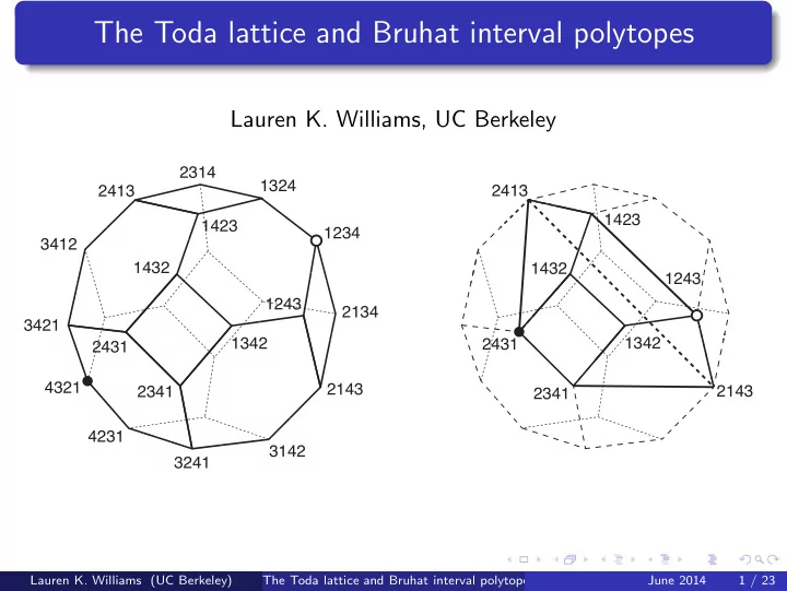
2314 1324 1234 2134 2143 1423 2413 3412 3421 4321 4231 3241 3142 1432 1342 1243 2431 2341 2143 1423 2413 1342 1243 2341 2431 1432
The Toda lattice and Bruhat interval polytopes
Lauren K. Williams, UC Berkeley
Lauren K. Williams (UC Berkeley) The Toda lattice and Bruhat interval polytopes June 2014 1 / 23