The story of the film so far... X , Y independent random variables - - PowerPoint PPT Presentation

SLIDE 1

Mathematics for Informatics 4a

Jos´ e Figueroa-O’Farrill Lecture 14 9 March 2012

Jos´ e Figueroa-O’Farrill mi4a (Probability) Lecture 14 1 / 23

The story of the film so far...

X, Y independent random variables and Z = X + Y: fZ = fX ⋆ fY, where ⋆ is the convolution X, Y with joint density f(x, y) and Z = g(X, Y): E(Z) =

• g(x, y)f(x, y)dx dy

X, Y independent:

E(XY) = E(X)E(Y)

Var(X + Y) = Var(X) + Var(Y)

MX+Y(t) = MX(t)MY(t), where MX(t) = E(etX)

We defined covariance and correlation of two r.v.s Proved Markov’s and Chebyshev’s inequalities Proved the (weak) law of large numbers and the Chernoff bound Waiting times of Poisson processes are exponentially distributed

Jos´ e Figueroa-O’Farrill mi4a (Probability) Lecture 14 2 / 23

More approximations

In Lecture 7 we saw that the binomial distribution with parameters n, p can be approximated by a Poisson distribution with parameter λ in the limit as n → ∞, p → 0 but np → λ:

n k

• pk(1 − p)n−k ∼ e−λ λk

k!

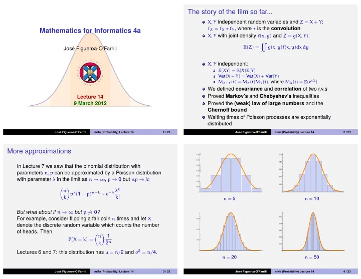
But what about if n → ∞ but p → 0? For example, consider flipping a fair coin n times and let X denote the discrete random variable which counts the number

• f heads. Then

P(X = k) = n k 1

2n Lectures 6 and 7: this distribution has µ = n/2 and σ2 = n/4.

Jos´ e Figueroa-O’Farrill mi4a (Probability) Lecture 14 3 / 23

0.05 0.10 0.15 0.20 0.25 0.30 0.35

n = 5

0.05 0.10 0.15 0.20 0.25

n = 10

0.05 0.10 0.15

n = 20

0.02 0.04 0.06 0.08 0.10

n = 50

Jos´ e Figueroa-O’Farrill mi4a (Probability) Lecture 14 4 / 23

SLIDE 2

Normal limit of (symmetric) binomial distribution

Theorem Let X be binomial with parameter n and p = 1

• 2. Then for n large

and k − n/2 not too large,

n k 1

2n ≃ 1

√

2πσ

e−(k−µ)2/2σ2 =

• 2

nπe−2(k−n/2)2/n

for µ = n/2 and σ2 = n/4. The proof rests on the de Moivre/Stirling formula for the factorial

• f a large number:

n! ≃ √

2πnn√ne−n which implies that

n n/2

• =

n! (n/2)!(n/2)! ≃ 2n

• 2

πn

Jos´ e Figueroa-O’Farrill mi4a (Probability) Lecture 14 5 / 23

Proof Let k = n

2 + x. Then

n k

• 2−n =
• n

n 2 + x

• 2−n =

n!2−n n

2 + x

! n

2 − x

! = n!2−n n

2

! n

2

! ×

n 2

n

2 − 1

• · · ·

n

2 − (x − 1)

• n

2 + 1

n

2 + 2

• · · ·

n

2 + x

• ≃
• 2

nπ ×

1

• 1 − 2

n

• · · ·
• 1 − (x − 1) 2

n

n

2

x

• 1 + 2

n

1 + 2 2

n

• · · ·
• 1 + x 2

n

n

2

x

Now we use the exponential approximation 1 − z ≃ e−z and 1 1 + z ≃ e−z (valid for z small) to rewrite the big fraction in the RHS.

Jos´ e Figueroa-O’Farrill mi4a (Probability) Lecture 14 6 / 23

Proof – continued.

n k

• 2−n ≃
• 2

nπ exp

• −4

n − 8 n − · · · − 2(x − 1) n − 2x n

• =
• 2

nπ exp

• −4

n(1 + 2 + · · · + (x − 1)) − 2x n

• =
• 2

nπ exp

• −4

n x(x − 1)

2

− 2x n

• =
• 2

nπe−2x2/n

which is indeed a normal distribution with σ2 = n

4 .

A similar proof shows that the general binomial distribution with

µ = np and σ2 = np(1 − p) is also approximated by a normal

distribution with the same µ and σ2.

Jos´ e Figueroa-O’Farrill mi4a (Probability) Lecture 14 7 / 23

Example (Rolling a die ad nauseam) It’s raining outside, you are bored and you roll a fair die 12000

• times. Let X be the number of sixes. What is

P(1900 < X < 2200)?

The variable X is the sum X1 + · · · + X12000, where Xi is the number of sixes on the ith roll. This means that X is binomially distributed with parameter n = 12000 and p = 1

6, so

µ = pn = 2000 and σ2 = np(1 − p) = 5000

3 .

X ∈ (1900, 2200) iff X−2000

σ

∈ (− √

6, 2

√

6), whence

P(1900 < X < 2200) ≃ Φ(2 √

6) − Φ(−

√

6) ≃ 0.992847 The exact result is

2199

• k=1901

12000 k

1 6

k

5 6

12000−k ≃ 0.992877

Jos´ e Figueroa-O’Farrill mi4a (Probability) Lecture 14 8 / 23

SLIDE 3

Normal limit of Poisson distribution

0.05 0.10 0.15

λ = 5

0.02 0.04 0.06 0.08 0.10 0.12

λ = 10

0.02 0.04 0.06 0.08

λ = 20

0.01 0.02 0.03 0.04 0.05

λ = 50

Jos´ e Figueroa-O’Farrill mi4a (Probability) Lecture 14 9 / 23

We have just shown that in certain limits of the defining parameters, two discrete probability distributions tend to normal distributions:

the binomial distribution in the limit n → ∞, the Poisson distribution in the limit λ → ∞

What about continuous probability distributions? We could try with the uniform or exponential distributions:

1 1 2 3 4 0.2 0.4 0.6 0.8 1.0 0.5 1.0 1.5 2.0 2.5 3.0 1 2 3 4

No amount of rescaling is going to work. Why?

Jos´ e Figueroa-O’Farrill mi4a (Probability) Lecture 14 10 / 23

The binomial and Poisson distributions have the following property:

if X, Y are binomially distributed with parameters (n, p) and

(m, p), X + Y is binomially distributed with parameter (n + m, p)

if X, Y are Poisson distributed with parameters λ and µ,

X + Y is Poisson distributed with parameter λ + µ

It follows that if X1, X2, . . . are i.i.d. with binomial distribution with parameters (m, p), X1 + · · · + Xn is binomial with parameter (nm, p). Therefore m large is equivalent to adding many of the Xi. It also follows that if X1, X2, . . . are i.i.d. with Poisson distribution with parameter λ, X1 + · · · + Xn is Poisson distributed with parameter nλ and again λ large is equivalent to adding a large number of the Xi. The situation with the uniform and exponential distributions is different.

Jos´ e Figueroa-O’Farrill mi4a (Probability) Lecture 14 11 / 23

Sum of uniformly distributed variables

Xi i.i.d. uniformly distributed on [0, 1]: then X1 + · · · + Xn is

1.0 0.5 0.5 1.0 1.5 2.0 0.2 0.4 0.6 0.8 1.0 1.2 1.4

n = 1

1 1 2 3 0.2 0.4 0.6 0.8 1.0

n = 2

1 1 2 3 4 0.2 0.4 0.6 0.8

n = 3

1 1 2 3 4 5 0.1 0.2 0.3 0.4 0.5 0.6 0.7

n = 4

Jos´ e Figueroa-O’Farrill mi4a (Probability) Lecture 14 12 / 23

SLIDE 4

Sum of exponentially distributed variables

If Xi are i.i.d. exponentially distributed with parameter λ, we already saw that Z2 = X1 + X2 has a “gamma” probability density function:

fZ2(z) = λ2ze−λz

It is not hard to show that Zn = X1 + · · · + Xn has probability density function

fZn(z) = λn zn−1 (n − 1)!e−λz

What happens when we take n large?

Jos´ e Figueroa-O’Farrill mi4a (Probability) Lecture 14 13 / 23

2 4 6 8 10 0.05 0.10 0.15

n = 5

5 10 15 20 0.02 0.04 0.06 0.08 0.10 0.12

n = 10

10 20 30 40 0.02 0.04 0.06 0.08

n = 20

20 40 60 80 100 120 140 0.01 0.02 0.03 0.04

n = 75

Jos´ e Figueroa-O’Farrill mi4a (Probability) Lecture 14 14 / 23

The Central Limit Theorem

Let X1, X2, . . . be i.i.d. random variables with mean µ and variance σ2. Let Zn = X1 + · · · + Xn. Then Zn has mean nµ and variance nσ2, but in addition we have Theorem (Central Limit Theorem) In the limit as n → ∞,

P Zn − nµ √nσ x

• → Φ(x)

with Φ the c.d.f. of the standard normal distribution. In other words, for n large, Zn is normally distributed.

Jos´ e Figueroa-O’Farrill mi4a (Probability) Lecture 14 15 / 23

Our 4-line proof of the CLT rests on L´ evy’s continuity law, which we will not prove. Paraphrasing: “the m.g.f. determines the c.d.f.” It is then enough to show that the limit n → ∞ of the m.g.f.

• f Zn−nµ

√nσ

is the m.g.f. of the standard normal distribution. Proof of CLT. We shift the mean: the variables Yi = Xi − µ are i.i.d. with mean 0 and variance σ2, and Zn − nµ = Y1 + · · · + Yn.

MZn−nµ(t) = MY1(t) · · · MYn(t) = MY1(t)n, by i.i.d. M Zn−nµ

√nσ (t) = MZn−nµ

• t

√nσ

• = MY1
• t

√nσ

n M Zn−nµ

√nσ (t) =

• 1 + σ2t2

2nσ2 + · · ·

n → et2/2, which is the m.g.f.

• f a standard normal variable.

Jos´ e Figueroa-O’Farrill mi4a (Probability) Lecture 14 16 / 23

SLIDE 5

Crucial observation The CLT holds regardless of how the Xi are distributed! The sum of any large number of i.i.d. normal variables always tends to a normal distribution. This also explains why normal distributions are so popular in probabilistic modelling. Let us look at a few examples.

Jos´ e Figueroa-O’Farrill mi4a (Probability) Lecture 14 17 / 23

Example (Rounding errors) Suppose that you round off 108 numbers to the nearest integer, and then add them to get the total S. Assume that the rounding errors are independent and uniform on [− 1

2, 1 2]. What is the

probability that S is wrong by more than 3? more than 6? Let Z = X1 + · · · + X108. We may approximate it by a normal distribution with µ = 0 and σ2 = 108

12 = 9, whence σ = 3.

S is wrong by more than 3 iff |Z| > 3 or |Z−µ|

σ

> 1 and hence P(|Z − µ| > σ) = 1 − P(|Z − µ| σ) = 1 − (2Φ(1) − 1) = 2(1 − Φ(1)) ≃ 0.3174 S is wrong by more than 6 iff |Z−µ|

σ

> 2 and hence P(|Z − µ| > 2σ) = 1 − P(|Z − µ| 2σ) = 1 − (2Φ(2) − 1) = 2(1 − Φ(2)) ≃ 0.0456

Jos´ e Figueroa-O’Farrill mi4a (Probability) Lecture 14 18 / 23

Place your bets!

Example (Roulette) A roulette wheel has 38 slots: the numbers 1 to 36 (18 black, 18 red) and the numbers 0 and 00 in green. You place a £1 bet on whether the ball will land on a red or black slot and win £1 if it does. Otherwise you lose the bet. Therefore you win £1 with probability

18 38 = 9 19 and you “win” −£1

with probability 20

38 = 10 19.

After 361 spins of the wheel, what is the probability that you are ahead? (Notice that 361 = 192.)

Jos´ e Figueroa-O’Farrill mi4a (Probability) Lecture 14 19 / 23

Example (Roulette – continued) Let Xi denote your winnings on the ith spin of the wheel. Then

P(Xi = 1) = 9

19 and P(Xi = −1) = 10

• 19. The mean is therefore

µ = P(Xi = 1) − P(Xi = −1) = − 1

19

and the variance is

σ2 = P(Xi = 1) + P(Xi = −1) − µ2 = 1 −

1 361 = 360 361

Then Z = X1 + · · · + X361 has mean −19 and variance 360. This means that after 361 spins you are down £19 on average. We are after the probability P(Z 0):

P(Z 0) = P

• Z+19

√ 360 19 √ 360

• = 1 − P
• Z+19

√ 360 19 √ 360

• ≃ 1 − Φ(1) ≃ 0.1587

So there is about a 16% chance that you are ahead.

Jos´ e Figueroa-O’Farrill mi4a (Probability) Lecture 14 20 / 23

SLIDE 6

Example (Measurements in astronomy) Astronomical measurements are subject to the vagaries of weather conditions and other sources of errors. Hence in order to estimate, say, the distance to a star one takes the average of many measurements. Let us assume that different measurements are i.i.d. with mean d (the distance to the star) and variance 4 (light-years2). How many measurements should we take to be “reasonably sure” that the estimated distance is accurate to within half a light-year? Let Xi denote the measurements and Zn = X1 + · · · + Xn. Let’s say that “reasonably sure” means 95%, which is 2σ in the standard normal distribution. (In Particle Physics, “reasonably sure” means 5σ, but this is Astronomy.) Then we are after n such that

P

• | Zn

n − d| 0.5

• ≃ 0.95

Jos´ e Figueroa-O’Farrill mi4a (Probability) Lecture 14 21 / 23

Example (Measurements in astronomy – continued) By the CLT we can assume that Zn−nd

2√n

is standard normal, so we are after

P

• | Zn−nd

2√n | √n 4

• ≃ 0.95
• r, equivalently,

√n 4

= 2, so that n = 64.

A question remains: is n = 64 large enough for the CLT? To answer it, we need to know more about the distribution of the

• Xi. However Chebyshev’s inequality can be used to provide a

safe n. Since E

• Zn

n

• = d and Var
• Zn

n

• = 4

n, Chebyshev’s

inequality says

P

• | Zn

n − d| > 0.5

• 4

n(0.5)2 = 16 n

so choosing n = 320 gives P

• | Zn

n − d| > 0.5

• 0.05 or

P

• | Zn

n − d| 0.5

• 0.95 as desired.

Jos´ e Figueroa-O’Farrill mi4a (Probability) Lecture 14 22 / 23

Summary

The binomial distribution with parameters n, p can be approximated by a normal distribution (with same mean and variance) for n large. Similarly for the Poisson distribution with parameter λ as

λ → ∞

These are special cases of the Central Limit Theorem: if

Xi are i.i.d. with mean µ and (nonzero) variance σ2, the

sum Zn = X1 + · · · + Xn for n large is normally distributed. We saw some examples on the use of the CLT: rounding errors, roulette game, astronomical measurements.

Jos´ e Figueroa-O’Farrill mi4a (Probability) Lecture 14 23 / 23