outline
play

Outline DM811 Fall 2009 Heuristics for Combinatorial Optimization - PowerPoint PPT Presentation

Outline DM811 Fall 2009 Heuristics for Combinatorial Optimization 1. Introduction Lecture 14 Race: A Configuration Tool 2. Inferential Statistics Basics of Inferential Statistics Experimental Designs Marco Chiarandini Deptartment of


  1. Outline DM811 – Fall 2009 Heuristics for Combinatorial Optimization 1. Introduction Lecture 14 Race: A Configuration Tool 2. Inferential Statistics Basics of Inferential Statistics Experimental Designs Marco Chiarandini Deptartment of Mathematics & Computer Science University of Southern Denmark 3. Race: Sequential Testing 2 Outline 
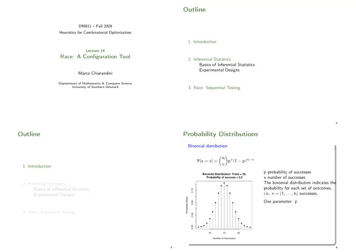
Probability Distributions Binomial distribution � n � p v ( 1 − p ) n − v P [ x = v ] = v 1. Introduction p probability of successes Binomial Distribution: Trials = 30, x number of successes Probability of success = 0.5 The binomial distribution indicates the 2. Inferential Statistics ● ● ● probability for each set of outcomes, Basics of Inferential Statistics 0.12 i.e. , v = { 1, . . . , n } successes. Experimental Designs ● ● Probability Mass One parameter: p 0.08 ● ● 3. Race: Sequential Testing ● ● 0.04 ● ● ● ● 0.00 ● ● ● ● ● ● 10 15 20 Number of Successes 3 4

  2. Uniform distribution (continuous) Normal distribution (continuous) 1 1 2σ2 ( x − µ ) 2 1 e − f ( x ) = f ( x ) = √ b − a σ 2π Theoretical importance Normal Distribution: µ = 0, σ = 1 Defined by two parameters: N ( µ, σ ) . 1.4 0.4 N ( 0, 1 ) is the standardized version. 1.2 0.3 In N ( 0, 1 ) 68.27 % of data fall within dunif(x, 0, 1) Density µ ± σ 0.2 1.0 0.1 0.8 0.0 0.6 −3 −2 −1 0 1 2 3 −0.5 0.0 0.5 1.0 1.5 x x <− seq(0, 1, by = 0.01) 5 6 Weibull distribution (continuous) Exponential distribution (continuous) � � β � t − γ � β − 1 f ( x ) = β t − γ f ( t ) = λe − λt e − η η η It has the memory-less property, i.e. , Exponential distribution: Weibull Distribution: the probability of a new event to Used in life data and reliability analysis lambda = 1 shape=1.5, scale=1, location=0 happen within a fixed time does not 1.0 Defined by three parameters: depend on the time passed so far. β (shape), η (scale), γ (location) 0.8 0.6 Defined by one parameter: E [ X ] = 1 λ . 0.6 Density Density 0.4 0.4 0.2 0.2 0.0 0.0 0 1 2 3 4 5 6 0 1 2 3 4 t t 7 8

  3. Outline Inferential Statistics We work with samples (instances, solution quality) But we want sound conclusions: generalization over a given population (all possible instances) 1. Introduction Thus we need statistical inference 2. Inferential Statistics Random Sample Population Inference Basics of Inferential Statistics X n P ( x, θ ) Experimental Designs Statistical Estimator � θ Parameter θ Since the analysis is based on finite-sized sampled data, statements like 3. Race: Sequential Testing “the cost of solutions returned by algorithm A is smaller than that of algorithm B ” must be completed by “at a level of significance of 5 % ”. 9 10 Parameter Estimation A Motivating Example θ ( X 1 , . . . , X n ) makes a guess on the parameter (Es. ¯ Estimator ^ There is a competition and two stochastic algorithms A 1 and A 2 are X ) submitted. Estimate is the actual value ^ θ ( x 1 , . . . , x n ) We run both algorithms once on n instances. Properties of an estimator: On each instance either A 1 wins (+) or A 2 wins (-) or they make a tie θ ] = θ ( e.g. , E [ ¯ unbiased: E [^ X ] = µ ) (=). consistent efficient (uncertainty must decrease with size, e.g. , Var [ ¯ X ] = σ 2 /n ) Questions: sufficient 1. If we have only 10 instances and algorithm A 1 wins 7 times how confident are we in claiming that algorithm A 1 is the best? Note: The best result b N = min i c i is not a good estimator. It is biased and 2. How many instances and how many wins should we observe to gain a not efficient. confidence of 95% that the algorithm A 1 is the best? 11 12

  4. A Motivating Example 1 If we have only 10 instances and algorithm A 1 wins 7 times how p : probability that A 1 wins on each instance (+) confident are we in claiming that algorithm A 1 is the best? n : number of runs without ties Y : number of wins of algorithm A 1 Under these conditions, we can check how unlikely the situation is if it were If each run is indepenedent and consitent: p (+) ≤ p (−) . � n � If p = 0.5 then the chance that algorithm A 1 wins 7 or more times out of 10 p y ( 1 − p ) n − y Pr [ Y = y ] = Y ∼ B ( n, p ) : y is 17.2 % : quite high! Binomial distribution: Trials = 30 Binomial Distribution: Trials = 30, Probability of success 0.5 0.25 Probability of success = 0.5 ● ● ● 0.20 0.12 ● ● Probability Mass 0.15 0.08 Pr[Y=y] ● ● 0.10 ● ● 0.04 0.05 ● ● ● ● 0.00 ● ● ● ● ● ● 0.00 10 15 20 0 2 4 6 8 10 number of successes y Number of Successes 13 14 Inferential Statistics 2 How many instances and how many wins should we observe to gain a General procedure: confidence of 95% that the algorithm A 1 is the best? Assume that data are consistent with a null hypothesis H 0 (e.g., sample data are drawn from distributions with the same mean value). To answer this question, we compute the 95 % quantile, i.e. , y : Pr [ Y ≥ y ] < 0.05 with p = 0.5 at different values of n : Use a statistical test to compute how likely this is to be true, given the data collected. This “likely” is quantified as the p-value. n 10 11 12 13 14 15 16 17 18 19 20 Accept H 0 as true if the p-value is larger than an user defined threshold y 9 9 10 10 11 12 12 13 13 14 15 called level of significance α . Alternatively (p-value < α ), H 0 is rejected in favor of an alternative hypothesis, H 1 , at a level of significance of α . This is an application example of sign test, a special case of binomial test in which p = 0.5 15 17

  5. Preparation of the Experiments Experimental Design Algorithms ⇒ Treatment Factor; Instances ⇒ Blocking Factor Variance reduction techniques Same pseudo random seed Design A: One run on various instances (Unreplicated Factorial) Algorithm 1 Algorithm 2 . . . Algorithm k Sample Sizes Instance 1 X 11 X 12 X 1k . . . . If the sample size is large enough (infinity) any difference in the means . . . . . . . . of the factors, no matter how small, will be significant Instance b X b1 X b2 X bk Real vs Statistical significance Study factors until the improvement in the response variable is deemed Design B: Several runs on various instances (Replicated Factorial) small Algorithm 1 Algorithm 2 . . . Algorithm k Desired statistical power + practical precision ⇒ sample size Instance 1 X 111 , . . . , X 11r X 121 , . . . , X 12r X 1k1 , . . . , X 1kr Instance 2 X 211 , . . . , X 21r X 221 , . . . , X 22r X 2k1 , . . . , X 2kr . . . . . . . . . . . . Note: If resources available for N runs then the optimal design is one run on Instance b X b11 , . . . , X b1r X b21 , . . . , X b2r X bk1 , . . . , X bkr N instances [Birattari, 2004] 19 20 Outline Unreplicated Designs Procedure Race [Birattari 2002] : 1. Introduction repeat Randomly select an unseen instance and run all candidates on it Perform all-pairwise comparison statistical tests Drop all candidates that are significantly inferior to the best algorithm 2. Inferential Statistics until only one candidate left or no more unseen instances ; Basics of Inferential Statistics Experimental Designs F-Race use Friedman test 3. Race: Sequential Testing Holm adjustment method is typically the most powerful 21 22

  6. Sequential Testing class−GEOMb (11 Instances) ... S_Seq_SL_Y O_DCFA O_DCFB O_CCFB S_RLF_Y O_CCFA S_RLF_N O_DRRB O_DRRA S_D_s_N O_CRRB O_DCRA O_CRRA S_D_g_N O_DCRB O_CCRA O_CCRB S_D_g_Y S_D_s_Y 0 1 2 3 4 5 6 7 8 9 10 11 12 13 14 15 16 17 18 Stage 24

Download Presentation
Download Policy: The content available on the website is offered to you 'AS IS' for your personal information and use only. It cannot be commercialized, licensed, or distributed on other websites without prior consent from the author. To download a presentation, simply click this link. If you encounter any difficulties during the download process, it's possible that the publisher has removed the file from their server.

Recommend


More recommend