1
play

1 A simplified definition Example: Rolling a dice Let be the - PDF document

Outline Probabilities Conditional probabilities Bayes theorem Distributions Discrete Continuous Advanced Herd Management Distribution functions Probabilities and distributions Sampling from distributions Estimation


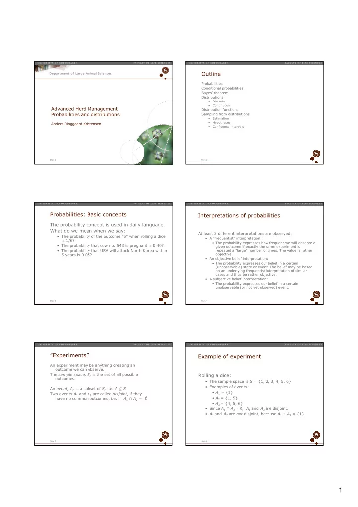
  1. Outline Probabilities Conditional probabilities Bayes’ theorem Distributions • Discrete • Continuous Advanced Herd Management Distribution functions Probabilities and distributions Sampling from distributions • Estimation • Hypotheses Anders Ringgaard Kristensen • Confidence intervals Slide 1 Slide 2 Probabilities: Basic concepts Interpretations of probabilities The probability concept is used in daily language. What do we mean when we say: At least 3 different interpretations are observed: • The probability of the outcome ”5” when rolling a dice • A “frequentist” interpretation: is 1/6? • The probability expresses how frequent we will observe a • The probability that cow no. 543 is pregnant is 0.40? given outcome if exactly the same experiment is • The probability that USA will attack North Korea within repeated a “large” number of times. The value is rather objective. 5 years is 0.05? • An objective belief interpretation: • The probability expresses our belief in a certain (unobservable) state or event. The belief may be based on an underlying frequentist interpretation of similar cases and thus be rather objective. • A subjective belief interpretation: • The probability expresses our belief in a certain unobservable (or not yet observed) event. Slide 3 Slide 4 ”Experiments” Example of experiment An experiment may be anything creating an outcome we can observe. The ���������������� is the set of all possible Rolling a dice: outcomes. • The sample space is � = {1, 2, 3, 4, 5, 6} • Examples of events: An ������ �� is a subset of �� i.e. �� ⊆ � • � 1 = {1} Two events � 1 and � 2 are called �������� , if they • � 2 = {1, 5} have no common outcomes, i.e. if � 1 � � 2 = ∅ • � 3 = {4, 5, 6} • Since � 1 � � 3 = ∅ , � 1 and � 3 are disjoint. • � 1 and � 2 are ��� disjoint, because � 1 ∩ � 2 = {1} Slide 5 Slide 6 1

  2. A simplified definition Example: Rolling a dice Let � be the sample space of an experiment. A probability distribution P on � is a function, Like before: � = {1, 2, 3, 4, 5, 6} so that A valid probability function on S is, for � ⊆ � : • P( � ) = 1. • P( � ) = | � |/6 where | � | is the size of � (i.e. the number of elements it contains) • For any event �� ∈ �� 0 ≤ P( � ) ≤ 1 • P({1}) = P({2}) = P({3}) = P({4}) = P({5}) = • For any two disjoint events � 1 and � 2 , P({6}) = 1/6 • P(A 1 ∪ A 2 ) = P(A 1 ) + P(A 2 ) • P({1, 5}) = 2/6 = 1/3 • P({1, 2, 3}) = 3/6 = 1/2 Notice, that many other valid probability functions could be defined (even though the one above is the only one that makes sense from a frequentist point of view). Slide 7 Slide 8 Conditional probabilities Independence Let � and � be two events, where P( � ) > 0 The ����������� probability of � given �� is If two events � and � are independent, then P( � � � ) = P( � )P( � ). written as P( � | � ), and it is by definition Example: Rolling two dices • � = {(1, 1), (1, 2),…, (1, 6),…, (6, 6)} • For any �� ⊆ � : P( � ) = | � |/36 • � = {(6, 1), (6, 2), …, (6, 6)} ⇒ P( � ) = 6/36 = 1/6 • � = {(1, 6), (2, 6), …, (6, 6)} ⇒ P( � ) = 6/36 = 1/6 • � � � = {(6, 6)} and P( � � ���� (1/6)(1/6) = 1/36 Slide 9 Slide 10 Example: Rolling a dice Conditional sum rule Again, let � = {1, 2, 3, 4, 5, 6}, and P( � ) = | � |/6. Let � 1 , � 2 , … � � be pair wise disjoint events Define � = {1, 2, 3}, and A = {2}. so that Then � � � = {2}, and Let �� be an event so that P( � ) > 0. Then The logical result: If you know the outcome is 1, 2 or 3, it is reasonable to assume that all 3 values are equally probable. Slide 11 Slide 12 2

  3. Bayes’ theorem Sum rule: Dice example Define the 3 disjoint events � 1 = {1, 2}, � 2 = Let A 1 , A 2 , … A n be pair wise disjoint events so {3, 4}, � 3 = {5, 6} that Thus � 1 ∪ � 2 ∪ � 3 = � Define ���� {1, 3, 5} (we know that P( � ) = ½) P( � | � 1 ) = P( � � � 1 )/P( � 1 ) = (1/6)/(1/3) = ½ Let B be an event so that P( B ) > 0. Then P( � | � 2 ) = P( � � � 2 )/P( � 2 ) = (1/6)/(1/3) = ½ P( � | � 3 ) = P( � � � 3 )/P( � 3 ) = (1/6)/(1/3) = ½ Thus Bayes’ theorem is extremely important in all kinds of reasoning under uncertainty. Updating of belief. Slide 13 Slide 14 Updating of belief, I Updating of belief, II In a dairy herd, the conception rate is known to be 0.40. Now, let us assume that the farmer observes the cow, and concludes, Define M as the event ”mating” for a cow. that it is not in heat. Define Π + as the event ”pregnant” for the same cow, and Π - as the Thus, we have observed the event H - and we would like to know the event ”not pregnant”. probability, that the cow is pregnant, i.e. we wish to calculate P( Π + | H - ) Thus P( Π + | M ) = 0.40 is a conditional probability. Given that the cow has been mated, the probability of pregnancy is 0.40. We apply Bayes’ theorem: Correspondingly, P( Π - | M ) = 0.60 After 3 weeks the farmer observes the cow for heat. The farmer’s heat detection rate is 0.55. Define H + as the event that the farmer detects heat. Thus, P( H + | Π - ) = We know all probabilities in the formula, and get 0.55, and P( H - | Π - ) = 0.45 There is a slight risk that the farmer erroneously observes a pregnant cow to be in heat. We assume, that P( H + | Π + ) = 0.01 Notice, that all probabilities are figures that makes sense and are In other words, our belief in the event ”pregnant” increases from 0.40 to estimated on a routine basis (except P( H + | Π + ) which is a guess) 0.59 based on a negative heat observation result Slide 15 Slide 16 Discrete distributions Summary of probabilities In some cases the probability is defined by a certain function defined over the Probabilities may be interpreted sample space. • As frequencies In those cases, we say that the outcome • As objective or subjective beliefs in certain events The belief interpretation enables us to represent uncertain is drawn from a standard distribution. knowledge in a concise way. There exist standard distributions for Bayes’ theorem lets us update our belief (knowledge) as new many natural phenomena. observations are done. If the sample space is a countable set, we denote the corresponding distribution as discrete. Slide 17 Slide 18 3

  4. Discrete distributions The binomial distribution I If �� is the random variable representing Consider an experiment with binary outcomes: the outcome, the expected value of a Success (s) or failure (f) discrete distribution is defined as • Mating of a sow → Pregnant (s), not pregnant (f) • Tossing a coin → Heads (s), tails (f) • Testing for a disease → Present (s), not present (f) Assume that the probability of success is � and The variance is defined as that the experiment is repeated �� times. Let � be the total number of successes observed in the � experiments. We shall look at two important discrete The sample space of the compound � experiments distributions: is � = {0, 1, 2, …, � } • The binomial distribution The ��������������� � is then said to be ���������� • The Poisson distribution. distributed with parameters � and � . Slide 19 Slide 20 The binomial distribution II The binomial distribution III The probability function P( � = � ) is (by The mean (expected value) of a binomial objective frequentist interpretation) distribution is simply E( � ) = �� . given by The variance is Var( � ) = �� (1M � ) The binomial distribution is one of the where most frequently used distribution for natural phenomena. is the �������������������� which may be calculated or looked up in a table. Slide 21 Slide 22 The Poisson distribution I The binomial distribution IV If a certain phenomenon occurs a random with a Three binomial distributions with n = 10 constant intensity (but independently of each others) the total number of occurrences � in a 0,35 0,3 time interval of a given length (or in a space of 0,25 a given area) is Poisson distributed with 0,2 0,2 P( k ) 0,5 parameter λ 0,15 0,8 0,1 Examples: 0,05 • Number of (nonMinfectious) disease cases per 0 month 0 1 2 3 4 5 6 7 8 9 10 k • Number of feeding system failures per year • Number of labor incidents per year Three binomial distributions, where ���� 10, and � = 0.2, 0.5 and 0.8, respectively. Slide 23 Slide 24 4

Download Presentation
Download Policy: The content available on the website is offered to you 'AS IS' for your personal information and use only. It cannot be commercialized, licensed, or distributed on other websites without prior consent from the author. To download a presentation, simply click this link. If you encounter any difficulties during the download process, it's possible that the publisher has removed the file from their server.

Recommend


More recommend