Dynamic Programming Greedy. Build up a solution incrementally, - - PowerPoint PPT Presentation

Dynamic Programming

Introduction, Weighted Interval Scheduling Tyler Moore

CSE 3353, SMU, Dallas, TX

Lecture 15

Some slides created by or adapted from Dr. Kevin Wayne. For more information see http://www.cs.princeton.edu/~wayne/kleinberg-tardos. Some code reused from Python Algorithms by Magnus Lie Hetland.

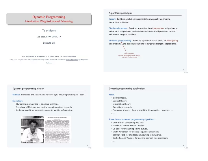
• Greedy. Build up a solution incrementally, myopically optimizing

some local criterion. Divide-and-conquer. Break up a problem into independent subproblems, solve each subproblem, and combine solution to subproblems to form solution to original problem. Dynamic programming. Break up a problem into a series of overlapping subproblems, and build up solutions to larger and larger subproblems.

2

fancy name for caching away intermediate results in a table for later reuse

2 / 28

• Bellman. Pioneered the systematic study of dynamic programming in 1950s.

Etymology.

Dynamic programming = planning over time. Secretary of Defense was hostile to mathematical research. Bellman sought an impressive name to avoid confrontation.

3

3 / 28

• Areas.

Bioinformatics. Control theory. Information theory. Operations research. Computer science: theory, graphics, AI, compilers, systems, …. ...

Some famous dynamic programming algorithms.

Unix diff for comparing two files. Viterbi for hidden Markov models. De Boor for evaluating spline curves. Smith-Waterman for genetic sequence alignment. Bellman-Ford for shortest path routing in networks. Cocke-Kasami-Younger for parsing context-free grammars. ...

4

4 / 28

Recurrence relations

Recall that recurrence relations are equations defined in terms of

• themselves. They are useful because many natural functions and

recursive functions can easily expressed as recurrences Recurrence Solution Example application T(n) = T(n/2) + 1 Θ(lg n) Binary Search T(n) = T(n/2) + n Θ(n) Randomized Quickselect (avg. case) T(n) = 2T(n/2) + 1 Θ(n) Tree traversal T(n) = 2T(n/2) + n Θ(n lg n) Mergesort T(n) = T(n − 1) + 1 Θ(n) Processing a sequence T(n) = T(n − 1) + n Θ(n2) Handshake problem T(n) = 2T(n − 1) + 1 Θ(2n) Towers of Hanoi T(n) = 2T(n − 1) + n Θ(2n) T(n) = nT(n − 1) Θ(n!)

5 / 28

Computing Fibonacci numbers

Fibonacci sequence can be defined using the following recurrence: Fn = Fn−1 + Fn−2, F0 = 0, F1 = 1 F2 = F1 + F0 = 1 + 0 = 1 F3 = F2 + F1 = 1 + 1 = 2 F4 = F3 + F2 = 2 + 1 = 3 F5 = F4 + F3 = 3 + 2 = 5 F6 = F5 + F4 = 5 + 3 = 8

6 / 28

Computing Fibonacci numbers with recursion

def f i b ( i ) : i f i < 2: return i return f i b ( i −1) + f i b ( i −2)

7 / 28

Recursion Tree for Fibonacci function

F(6) F(5) F(4) F(3) F(2) F(1) F(0) F(1) F(2) F(1) F(0) F(3) F(2) F(1) F(0) F(1) F(4) F(3) F(2) F(1) F(0) F(1) F(2) F(1) F(0)

We know that T(n) = 2T(n − 1) + 1 = Θ(2n) It turns out that T(n) = T(n − 1) + T(n − 2) ≈ Θ(1.6n) Since our recursion tree has 0 and 1 as leaves, computing Fn requires ≈ 1.6n recursive function calls!

8 / 28

Computing Fibonacci numbers with memoization (manual)

def fib memo ( i ) : mem = {} #d i c t

• f

cached v a l u e s def f i b ( x ) : i f x < 2: return x #check i f a l r e a d y computed i f x in mem: return mem[ x ] #only i f not a l r e a d y computed mem[ x ] = f i b ( x−1) + f i b ( x−2) return mem[ x ] f i b ( i ) return mem[ i ]

9 / 28

Recursion tree for Fibonacci function with memoization

F(6) F(5) F(4) F(3) F(2) F(1) F(0) F(1) F(2) F(1) F(0) F(3) F(2) F(1) F(0) F(1) F(4) F(3) F(2) F(1) F(0) F(1) F(2) F(1) F(0)

Black nodes: no longer computed due to memoization Caching reduced the # of operations from exponential to linear time!

10 / 28

Computing Fibonacci numbers with memoization (automatic)

> > > @memo . . . def f i b ( i ) : . . . i f i < 2: return i . . . return f i b ( i −1) + f i b ( i −2) . . . > > > f i b (100) 354224848179261915075L What sort of magic is going on here?

11 / 28

Code for the memo wrapper

from f u n c t o o l s import wraps def memo( func ) : cache = {} # Stored subproblem s o l u t i o n s @wraps ( func ) # Make wrap look l i k e func def wrap (∗ args ) : # The memoized wrapper i f args not in cache : # Not a l r e a d y computed? cache [ args ] = func (∗ args ) # Compute & cache the s o l u t i o n return cache [ args ]# Return the cached s o l u t i o n return wrap # Return the wrapper Example of Python’s capability as a functional language Provides cache functionality for recursive functions in general The memo function takes a function as input, then “wraps the function with the added functionality The @wraps statement makes the memo function a decorator

12 / 28

Discussion of dynamic memoization

Even if the code is a bit of a mystery, don’t worry, you can still use it by including the code on the last slide with yours, then making the first line before your function definition decorated by ‘@memo’ If you don’t have access to a programming language supporting dynamic memoization, you can either do it manually or turn to dynamic programming Dynamic programming converts recursive code to an iterative version that executes efficiently

13 / 28

Computing Fibonacci numbers with dynamic programming

def f i b i t e r ( i ) : i f i < 2: return i #s t o r e the sequence in a l i s t mem=[0 ,1] for j in range (2 , i +1): #i n c r e m e n t a l l y b u i l d the sequence

• mem. append (mem[ j −1]+mem[ j −2])

return mem[ −1]

14 / 28

Avoiding recomputation by storing partial results

The trick to dynamic programming is to see that the naive recursive algorithm repeatedly computes the same subproblems over and over and over again. If so, storing the answers to them in a table instead

• f recomputing can lead to an efficient algorithm.

Thus we must first hunt for a correct recursive algorithm – later we can worry about speeding it up by using a results matrix.

15 / 28

• 6. DYNAMIC PROGRAMMING I
• weighted interval scheduling
• segmented least squares
• knapsack problem
• RNA secondary structure

16 / 28

• Weighted interval scheduling problem.

Job starts at , finishes at , and has weight or value . Two jobs compatible if they don't overlap. Goal: find maximum weight subset of mutually compatible jobs.

6

• f

g h e a b c d

1 2 3 4 5 6 7 8 9 10 11

17 / 28

• Earliest finish-time first.

Consider jobs in ascending order of finish time. Add job to subset if it is compatible with previously chosen jobs.

• Recall. Greedy algorithm is correct if all weights are 1.
• Observation. Greedy algorithm fails spectacularly for weighted version.

7

weight = 999 weight = 1

• 1

2 3 4 5 6 7 8 9 10 11

b a h 18 / 28

• Notation. Label jobs by finishing time: ≤≤≤.
• Def. largest index such that job is compatible with .

Ex.

• 8
• 1

2 3 4 5 6 7 8 9 10 11

6 7 8 4 3 1 2 5 19 / 28

• Notation. value of optimal solution to the problem consisting of

job requests . Case 1. selects job .

Collect profit . Can't use incompatible jobs . Must include optimal solution to problem consisting of remaining

compatible jobs . Case 2. does not select job .

Must include optimal solution to problem consisting of remaining

compatible jobs .

• −
• ⎧

⎨ ⎩

9

• ptimal substructure property

(proof via exchange argument)

20 / 28

• 10

Input: n, s[1..n], f[1..n], v[1..n] Sort jobs by finish time so that f[1] ≤ f[2] ≤ … ≤ f[n]. Compute p[1], p[2], …, p[n]. Compute-Opt(j) if j = 0 return 0. else return max(v[j] + Compute-Opt(p[j], Compute-Opt(j–1))).

21 / 28

• Observation. Recursive algorithm fails spectacularly because of redundant

subproblems ⇒ exponential algorithms.

• Ex. Number of recursive calls for family of "layered" instances grows like

Fibonacci sequence.

11

3 4 5 1 2

• 5

4 3 3 2 2 1 1 1 1 1 1

• 22 / 28
• Memoization. Cache results of each subproblem; lookup as needed.

global array

• 12

Input: n, s[1..n], f[1..n], v[1..n] Sort jobs by finish time so that f[1] ≤ f[2] ≤ … ≤ f[n]. Compute p[1], p[2], …, p[n]. for j = 1 to n M[j] ← empty. M[0] ← 0. M-Compute-Opt(j) if M[j] is empty M[j] ← max(v[j] + M-Compute-Opt(p[j]), M-Compute-Opt(j – 1)). return M[j].

23 / 28

• Claim. Memoized version of algorithm takes time.

Sort by finish time: . Computing ⋅ : via sorting by start time. : each invocation takes time and either

(i) returns an existing value M[j] (ii) fills in one new entry M[j] and makes two recursive calls

Progress measure Φ nonempty entries of M[].

initially Φ, throughout Φ≤. (ii) increases Φ by ⇒ at most recursive calls.

Overall running time of is . ▪

• Remark. if jobs are presorted by start and finish times.

13

24 / 28

• Bottom-up dynamic programming. Unwind recursion.

15

• ≤≤≤
• ←
• ←
• 25 / 28

Weighted Interval Scheduling Example

Index 1 2 3 4 5 6 v1 = 2 v2 = 4 v3 = 4 v4 = 7 v5 = 2 v6 = 1

j vj p(j) vj + M[p(j)] M[j − 1] M[j] 1 2 2 + 0 2 2 4 4 + 0 2 4 3 4 1 4 + 2 4 6 4 7 7 + 0 6 7 5 2 3 2 + 6 7 8 6 1 3 1 + 6 8 8

26 / 28

Weighted Interval Scheduling Exercise

Index 1 2 3 4 5 v1 = 2 v2 = 3 v3 = 6 v4 = 1 v5 = 9

j vj p(j) vj + M[p(j)] M[j − 1] M[j] 1 2 2 3 3 6 4 1 5 9

27 / 28

• Q. DP algorithm computes optimal value. How to find solution itself?
• A. Make a second pass.
• Analysis. # of recursive calls ≤⇒.

14

Find-Solution(j) if j = 0 return ∅. else if (v[j] + M[p[j]] > M[j–1]) return ∪ Find-Solution(p[j]). else return Find-Solution(j–1).

28 / 28