The phase transition for level sets of smooth planar Gaussian fields - - PowerPoint PPT Presentation

The phase transition for level sets

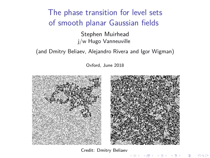
• f smooth planar Gaussian fields

Stephen Muirhead

j/w Hugo Vanneuville (and Dmitry Beliaev, Alejandro Rivera and Igor Wigman)

Oxford, June 2018 Credit: Dmitry Beliaev

Gaussian fields and percolation

The conjecture: Under mild conditions, the connectivity of the level sets of smooth, stationary Gaussian fields ‘behaves like’ Bernoulli percolation.

2 34

Gaussian fields and percolation

The conjecture: Under mild conditions, the connectivity of the level sets of smooth, stationary Gaussian fields ‘behaves like’ Bernoulli percolation. Two main aspects to this conjecture:

2 34

Gaussian fields and percolation

The conjecture: Under mild conditions, the connectivity of the level sets of smooth, stationary Gaussian fields ‘behaves like’ Bernoulli percolation. Two main aspects to this conjecture:

◮ Existence and sharpness of the phase transition (exponential

decay of crossing probabilities, polynomial critical window).

2 34

Gaussian fields and percolation

The conjecture: Under mild conditions, the connectivity of the level sets of smooth, stationary Gaussian fields ‘behaves like’ Bernoulli percolation. Two main aspects to this conjecture:

◮ Existence and sharpness of the phase transition (exponential

decay of crossing probabilities, polynomial critical window).

◮ Scaling limits at the critical level (RSW estimates,

convergence of crossing probabilities, convergence to CLE).

2 34

Gaussian fields and percolation

Let f be a stationary, centred, continuous Gaussian field on R2 with covariance kernel κ(x) = E[f (0)f (x)] , x ∈ R2.

3 34

Gaussian fields and percolation

Let f be a stationary, centred, continuous Gaussian field on R2 with covariance kernel κ(x) = E[f (0)f (x)] , x ∈ R2. Define the level sets and (lower-)excursion sets of f by Lℓ = {x : f (x) = ℓ} and Eℓ = {x : f (x) ≤ ℓ}.

3 34

Gaussian fields and percolation

Let f be a stationary, centred, continuous Gaussian field on R2 with covariance kernel κ(x) = E[f (0)f (x)] , x ∈ R2. Define the level sets and (lower-)excursion sets of f by Lℓ = {x : f (x) = ℓ} and Eℓ = {x : f (x) ≤ ℓ}. We say that Lℓ or Eℓ percolate if almost surely they have an unbounded connected component.

3 34

Gaussian fields and percolation

By monotonicity, there exists a critical level ℓc ∈ [−∞, ∞] such that Eℓ percolates if ℓ > ℓc and does not if ℓ < ℓc.

4 34

Gaussian fields and percolation

By monotonicity, there exists a critical level ℓc ∈ [−∞, ∞] such that Eℓ percolates if ℓ > ℓc and does not if ℓ < ℓc. Under mild conditions on κ it is natural to expect that ℓc = 0.

4 34

Gaussian fields and percolation

By monotonicity, there exists a critical level ℓc ∈ [−∞, ∞] such that Eℓ percolates if ℓ > ℓc and does not if ℓ < ℓc. Under mild conditions on κ it is natural to expect that ℓc = 0. In fact, we expect a phase transition at ℓc = 0 :

◮ If ℓ ≤ 0, then almost surely the connected components of Eℓ

are bounded;

◮ If ℓ > 0, then almost surely Eℓ has a unique unbounded

connected component.

4 34

Previous results

In 1983, Molchanov & Stepanov showed that if κ is absolutely integrable then ℓc < ∞, i.e., there exists a ℓ∗ < ∞ such that Eℓ percolates at every level ℓ ≥ ℓ∗.

5 34

Previous results

In 1983, Molchanov & Stepanov showed that if κ is absolutely integrable then ℓc < ∞, i.e., there exists a ℓ∗ < ∞ such that Eℓ percolates at every level ℓ ≥ ℓ∗. In 1996, Alexander showed that if f is ergodic and κ is positive then the connected components of the level sets are a.s. bounded.

5 34

Previous results

In 1983, Molchanov & Stepanov showed that if κ is absolutely integrable then ℓc < ∞, i.e., there exists a ℓ∗ < ∞ such that Eℓ percolates at every level ℓ ≥ ℓ∗. In 1996, Alexander showed that if f is ergodic and κ is positive then the connected components of the level sets are a.s. bounded. By the symmetry (in law) of the positive and negative excursion sets, this implies that ℓc ≥ 0.

5 34

Previous results

In 1983, Molchanov & Stepanov showed that if κ is absolutely integrable then ℓc < ∞, i.e., there exists a ℓ∗ < ∞ such that Eℓ percolates at every level ℓ ≥ ℓ∗. In 1996, Alexander showed that if f is ergodic and κ is positive then the connected components of the level sets are a.s. bounded. By the symmetry (in law) of the positive and negative excursion sets, this implies that ℓc ≥ 0. Together, these results show that if correlations are (i) positive, and (iii) integrable, then 0 ≤ ℓc < ∞.

5 34

Previous results

Recently, advances in percolation theory have inspired a flurry of new results:

◮ In 2016, Beffara & Gayet proved that, if κ is (i) positive,

(ii) symmetric, and (iii) decays polynomially with exponent γ > 325, then the ‘RSW estimates’ hold at the zero level.

6 34

Previous results

Recently, advances in percolation theory have inspired a flurry of new results:

◮ In 2016, Beffara & Gayet proved that, if κ is (i) positive,

(ii) symmetric, and (iii) decays polynomially with exponent γ > 325, then the ‘RSW estimates’ hold at the zero level.

◮ The necessary exponent γ for RSW estimates has been

subsequently reduced, first to γ > 16 [Beliaev & M, 2017], then to γ > 4 [Rivera & Vanneuville, 2017] (integrability corresponds to γ > 2).

6 34

Previous results

◮ It was also recently shown [Rivera & Vanneuville, 2017] that

the phase transition exists for the Bargmann-Fock field, i.e. the Gaussian field with covariance κ(x) = e−|x|2/2. Their argument relied on exact Fourier-type computations on the covariance kernel κ.

7 34

Our results

8 34

Our results

Let µ denote the spectral measure, defined via: κ(x) =

• e2πix,s dµ(s).

8 34

Our results

Let µ denote the spectral measure, defined via: κ(x) =

• e2πix,s dµ(s).

We always work under the assumption that µ is absolutely continuous (w.r.t. dx); we denote by ρ2 the density of µ.

8 34

Our results

Let µ denote the spectral measure, defined via: κ(x) =

• e2πix,s dµ(s).

We always work under the assumption that µ is absolutely continuous (w.r.t. dx); we denote by ρ2 the density of µ. The existence of the spectral density guarantees that f is non-degenerate and ergodic, and also that κ(x) → 0 as |x| → ∞.

8 34

Our results

Let µ denote the spectral measure, defined via: κ(x) =

• e2πix,s dµ(s).

We always work under the assumption that µ is absolutely continuous (w.r.t. dx); we denote by ρ2 the density of µ. The existence of the spectral density guarantees that f is non-degenerate and ergodic, and also that κ(x) → 0 as |x| → ∞. On the other hand, this assumption is weaker than the condition that the covariance kernel κ is absolutely integrable, and also holds for the band-limited kernels.

8 34

Our results

The existence of the spectral density is fundamental to our analysis because it permits a white-noise representation of f : f

d

= q ⋆ W where q := F[ρ] ∈ L2(R2), W is a planar white-noise, and ⋆ denotes convolution.

9 34

Our results

The existence of the spectral density is fundamental to our analysis because it permits a white-noise representation of f : f

d

= q ⋆ W where q := F[ρ] ∈ L2(R2), W is a planar white-noise, and ⋆ denotes convolution. To see why this is true, consider that q ⋆ W is a stationary Gaussian field with covariance kernel q ⋆ q = F[ρ] ⋆ F[ρ] = F[ρ2] = κ.

9 34

Our results

The existence of the spectral density is fundamental to our analysis because it permits a white-noise representation of f : f

d

= q ⋆ W where q := F[ρ] ∈ L2(R2), W is a planar white-noise, and ⋆ denotes convolution. To see why this is true, consider that q ⋆ W is a stationary Gaussian field with covariance kernel q ⋆ q = F[ρ] ⋆ F[ρ] = F[ρ2] = κ. In fact, the existence of this representation is equivalent to the existence of ρ2.

9 34

Our results: Assumptions

Our results hold under the following additional assumptions on q:

10 34

Our results: Assumptions

Our results hold under the following additional assumptions on q:

◮ (Regularity) The function q is in C3;

10 34

Our results: Assumptions

Our results hold under the following additional assumptions on q:

◮ (Regularity) The function q is in C3; ◮ (Symmetry) The function q is symmetric under (i) reflection

in the x-axis, and (ii) rotation by π/2 about the origin.

10 34

Our results: Assumptions

Our results hold under the following additional assumptions on q:

◮ (Regularity) The function q is in C3; ◮ (Symmetry) The function q is symmetric under (i) reflection

in the x-axis, and (ii) rotation by π/2 about the origin.

◮ (Positivity) The function q ≥ 0 is positive.

10 34

Our results: Assumptions

Our results hold under the following additional assumptions on q:

◮ (Regularity) The function q is in C3; ◮ (Symmetry) The function q is symmetric under (i) reflection

in the x-axis, and (ii) rotation by π/2 about the origin.

◮ (Positivity) The function q ≥ 0 is positive. ◮ (‘Integrable correlations’) There exists γ > 2 and c > 0 such

that, for every |x| > 1, |q(x)| < c|x|−γ, and, for every multi-index α such that |α| ≤ 2, |∂αq(x)| < c|x|−γ.

10 34

Our results: Existence of the phase transition

Our first result confirms the phase transition at the zero level:

11 34

Our results: Existence of the phase transition

Our first result confirms the phase transition at the zero level:

Theorem

Under the stated conditions:

◮ If ℓ ≤ 0, then almost surely the connected components of Eℓ

are bounded;

◮ If ℓ > 0, then almost surely Eℓ has a unique unbounded

connected component.

11 34

Our results: Existence of the phase transition

Another way to state this result is in terms of the ‘ε’-thickened nodal set:

Theorem

Let Nε = {|f | ≤ ε}. Then under the stated conditions:

◮ If ε = 0, then almost surely the connected components of Nε

are bounded;

◮ If ε > 0, then almost surely Nε has a unique unbounded

connected component.

12 34

Our results: Sharpness of the phase transition

Our next result establishes that the phase transition is sharp (i.e. sub-critical crossing probabilities decay rapidly).

13 34

Our results: Sharpness of the phase transition

Our next result establishes that the phase transition is sharp (i.e. sub-critical crossing probabilities decay rapidly). Define a quad Q to be a simply-connected piece-wise smooth compact domain D ⊂ R2 and two disjoint boundary arcs η and η′. One can take, for instance, D to be a rectangle and η and η′ to be

• pposite edges.

13 34

Our results: Sharpness of the phase transition

Our next result establishes that the phase transition is sharp (i.e. sub-critical crossing probabilities decay rapidly). Define a quad Q to be a simply-connected piece-wise smooth compact domain D ⊂ R2 and two disjoint boundary arcs η and η′. One can take, for instance, D to be a rectangle and η and η′ to be

• pposite edges.

For each quad Q and level ℓ, let Crossℓ(Q) denote the event that there is a connected component of Eℓ that crosses Q, i.e., whose intersection with Q intersects both η and η′.

13 34

Our results: Sharpness of the phase transition

Theorem

Under the stated conditions, the following hold for every Q:

◮ If ℓ < 0, there exist c1, c2 > 0 such that, for all s ≥ 1,

P (f ∈ Crossℓ(sQ)) < c1e−c2 log2(s).

14 34

Our results: Sharpness of the phase transition

Theorem

Under the stated conditions, the following hold for every Q:

◮ If ℓ < 0, there exist c1, c2 > 0 such that, for all s ≥ 1,

P (f ∈ Crossℓ(sQ)) < c1e−c2 log2(s).

◮ If ℓ = 0,

inf

s>0 P(f ∈ Cross0(sQ)) > 0

and sup

s>0

P(f ∈ Cross0(sQ)) < 1.

14 34

Our results: Sharpness of the phase transition

Theorem

Under the stated conditions, the following hold for every Q:

◮ If ℓ < 0, there exist c1, c2 > 0 such that, for all s ≥ 1,

P (f ∈ Crossℓ(sQ)) < c1e−c2 log2(s).

◮ If ℓ = 0,

inf

s>0 P(f ∈ Cross0(sQ)) > 0

and sup

s>0

P(f ∈ Cross0(sQ)) < 1.

◮ If ℓ > 0, there exist c1, c2 > 0 such that, for all s ≥ 1,

P (f ∈ Crossℓ(sQ)) > 1 − c1e−c2 log2(s).

14 34

Our results: Sharpness of the phase transition

We can show exponential decay of crossing probabilities if we additionally assume ‘strong-exponential’ decay of correlations.

15 34

Our results: Sharpness of the phase transition

We can show exponential decay of crossing probabilities if we additionally assume ‘strong-exponential’ decay of correlations.

Theorem

Suppose that, in addition to the above assumptions, there exists a constant c > 0 such that, for every |x| > 1 and for every multi-index α such that |α| ≤ 2, |∂αq(x)| < ce−|x|(log |x|)2. Then, for each ℓ < 0 there exist c1, c2 > 0 such that, for all s ≥ 1, P (f ∈ Crossℓ(sQ)) < c1e−c2s.

15 34

Our results: The near-critical window

Our final results concerns the size of the near-critical window.

16 34

Our results: The near-critical window

Our final results concerns the size of the near-critical window. The previous result implied that, for fixed ℓ > 0 P [f ∈ Crossℓ(sQ)] → 1 as s → ∞.

16 34

Our results: The near-critical window

Our final results concerns the size of the near-critical window. The previous result implied that, for fixed ℓ > 0 P [f ∈ Crossℓ(sQ)] → 1 as s → ∞. How quickly we can take ℓs → 0 so that the above still holds?

16 34

Our results: The near-critical window

Our final results concerns the size of the near-critical window. The previous result implied that, for fixed ℓ > 0 P [f ∈ Crossℓ(sQ)] → 1 as s → ∞. How quickly we can take ℓs → 0 so that the above still holds?

Theorem

Under the stated conditions, there exist 0 < c1 < c2 < ∞ such that, for every quad Q, lim sup

s→∞

P [f ∈ Crosss−c2(sQ)] < 1 and lim

s→∞ P [f ∈ Crosss−c1(sQ)] = 1.

16 34

Our results: The near-critical window

By analogy with Bernoulli percolation, we conjecture that the near-critical window is of polynomial size with exponent exactly 3/4.

17 34

Our results: The near-critical window

By analogy with Bernoulli percolation, we conjecture that the near-critical window is of polynomial size with exponent exactly 3/4. We can show only that it is strictly positive and at most 1 (which is roughly all that is known in percolation outside some special lattices).

17 34

The percolation universality class

A major unresolved question raised by our work is to determine how rapidly correlations must decay in order for the analogy with percolation to be valid. That is, for which κ do our results hold (and more refined results, such as the convergence of the nodal set to CLE(6))?

18 34

The percolation universality class

According to the ‘Harris criterion’, the percolation universality class consists of all κ satisfying

• x∈BR
• y∈BR

κ(x − y) dxdy ≪ R5/2; for positive κ, this equates to polynomial decay of order γ > 3/2.

19 34

The percolation universality class

According to the ‘Harris criterion’, the percolation universality class consists of all κ satisfying

• x∈BR
• y∈BR

κ(x − y) dxdy ≪ R5/2; for positive κ, this equates to polynomial decay of order γ > 3/2. The random plane wave satisfies the HC since

• x∈BR
• y∈BR

J0(|x − y|) dxdy = O(R). despite correlations decaying only at rate R−1/2 (for which the LHS is a priori O(R7/2))

19 34

Elements of the proof

The proof consists of four steps:

20 34

Elements of the proof

The proof consists of four steps:

• 1. (Quasi-independence) Show that crossing events on domains
• f scale R separated by a distance R are asymptotically

independent as R → ∞;

20 34

Elements of the proof

The proof consists of four steps:

• 1. (Quasi-independence) Show that crossing events on domains
• f scale R separated by a distance R are asymptotically

independent as R → ∞;

• 2. (RSW estimates) Apply a general argument of Tassion to

deduce the RSW estimates at the zero level ℓ = 0;

20 34

Elements of the proof

The proof consists of four steps:

• 1. (Quasi-independence) Show that crossing events on domains
• f scale R separated by a distance R are asymptotically

independent as R → ∞;

• 2. (RSW estimates) Apply a general argument of Tassion to

deduce the RSW estimates at the zero level ℓ = 0;

• 3. (ℓc = 0) Use ideas from randomised algorithms (i.e. the OSSS

inequality) to deduce a qualitative description of the phase transition at ℓ = 0.

20 34

Elements of the proof

The proof consists of four steps:

• 1. (Quasi-independence) Show that crossing events on domains
• f scale R separated by a distance R are asymptotically

independent as R → ∞;

• 2. (RSW estimates) Apply a general argument of Tassion to

deduce the RSW estimates at the zero level ℓ = 0;

• 3. (ℓc = 0) Use ideas from randomised algorithms (i.e. the OSSS

inequality) to deduce a qualitative description of the phase transition at ℓ = 0.

• 4. (Sharpness) Bootstrap the previous step to give a quantitative

description of the phase transition.

20 34

Elements of the proof: Quasi-independence

To prove QI, we couple f to the R-dependent field fR = qR ⋆ W = (qχR) ⋆ W where χR is a smooth approximation of x → ✶|x|≤R/2.

21 34

Elements of the proof: Quasi-independence

To prove QI, we couple f to the R-dependent field fR = qR ⋆ W = (qχR) ⋆ W where χR is a smooth approximation of x → ✶|x|≤R/2. Then, under this coupling, f − fR = (q − qR) ⋆ W is a stationary Gaussian field with covariance (q − qR) ⋆ (q − qR).

21 34

Elements of the proof: Quasi-independence

To prove QI, we couple f to the R-dependent field fR = qR ⋆ W = (qχR) ⋆ W where χR is a smooth approximation of x → ✶|x|≤R/2. Then, under this coupling, f − fR = (q − qR) ⋆ W is a stationary Gaussian field with covariance (q − qR) ⋆ (q − qR). Standard arguments (Kolmogorov, BTIS) then give that P[|f − fR|C0(BR) > ε] < δ for ε ≈ R1−γ and δ ≈ e−c2(log R)2.

21 34

Elements of the proof: Quasi-independence

Since crossing events separated by a distance R are independent for fR, it remains to find a bound on |P[f ∈ Crossℓ(RQ)] − P[fR ∈ Crossℓ(RQ)]|.

22 34

Elements of the proof: Quasi-independence

Since crossing events separated by a distance R are independent for fR, it remains to find a bound on |P[f ∈ Crossℓ(RQ)] − P[fR ∈ Crossℓ(RQ)]|. By monotonicity and the bound on f − fRC0(BR), it is enough to find a bound on |P[f ∈ Crossℓ(RQ)] − P[f ± ε ∈ Crossℓ(RQ)]| for ε ≈ R1−γ.

22 34

We use a general approach based on the Cameron-Martin theorem:

23 34

We use a general approach based on the Cameron-Martin theorem:

Theorem (Cameron–Martin)

Let H be the RKHS of f . Then for every h ∈ H, the Radon–Nikodym derivative of the law of f + h with respect to the law of f is exp

• f , h − 1

2E[f , h2]

• .

where f , h is the ‘Paley-Weiner integral’.

23 34

We use a general approach based on the Cameron-Martin theorem:

Theorem (Cameron–Martin)

Let H be the RKHS of f . Then for every h ∈ H, the Radon–Nikodym derivative of the law of f + h with respect to the law of f is exp

• f , h − 1

2E[f , h2]

• .

where f , h is the ‘Paley-Weiner integral’.

Corollary

For every h ∈ H and event A, |P[f ∈ A] − P[f ± h ∈ A]| ≤ hH

• P [f ∈ A]

√log 2 .

23 34

Elements of the proof: Quasi-independence

Recall that the RKHS can be represented as H = F[gρ] , g ∈ L2

sym(R2).

✶

24 34

Elements of the proof: Quasi-independence

Recall that the RKHS can be represented as H = F[gρ] , g ∈ L2

sym(R2).

This gives the identity h2

H =

• x∈R2 |ˆ

h(x)|2/ρ2(x) dx, which means that, if h ≈ ✶BR, then h2

H ≈

• x∈B(1/R) ρ−2(x) dx.

24 34

Elements of the proof: Quasi-independence

Recall that the RKHS can be represented as H = F[gρ] , g ∈ L2

sym(R2).

This gives the identity h2

H =

• x∈R2 |ˆ

h(x)|2/ρ2(x) dx, which means that, if h ≈ ✶BR, then h2

H ≈

• x∈B(1/R) ρ−2(x) dx.

Proposition

Suppose ρ(0) > 0. Then there exist c, R0 > 0 such that, for every R > R0, monotonic event A that depends on f |BR, and ε > 0, |P [f ∈ A] − P[f ± ε ∈ A]| ≤ cRε

• P [f ∈ A].

24 34

Elements of the proof: Quasi-independence

Recall that the RKHS can be represented as H = F[gρ] , g ∈ L2

sym(R2).

This gives the identity h2

H =

• x∈R2 |ˆ

h(x)|2/ρ2(x) dx, which means that, if h ≈ ✶BR, then h2

H ≈

• x∈B(1/R) ρ−2(x) dx.

Proposition

Suppose ρ(0) > 0. Then there exist c, R0 > 0 such that, for every R > R0, monotonic event A that depends on f |BR, and ε > 0, |P [f ∈ A] − P[f ± ε ∈ A]| ≤ cRε

• P [f ∈ A].

From here, it is easy to deduce QI if γ > 2,

24 34

Elements of the proof: RSW estimates

To prove RSW estimates we borrow an argument of Tassion that applies to any stationary random colouring of the plane with three key properties:

25 34

Elements of the proof: RSW estimates

To prove RSW estimates we borrow an argument of Tassion that applies to any stationary random colouring of the plane with three key properties:

◮ Sufficient symmetry, guaranteed by our assumptions;

25 34

Elements of the proof: RSW estimates

To prove RSW estimates we borrow an argument of Tassion that applies to any stationary random colouring of the plane with three key properties:

◮ Sufficient symmetry, guaranteed by our assumptions; ◮ The QI property; and

25 34

Elements of the proof: RSW estimates

To prove RSW estimates we borrow an argument of Tassion that applies to any stationary random colouring of the plane with three key properties:

◮ Sufficient symmetry, guaranteed by our assumptions; ◮ The QI property; and ◮ Positive associations, which is equivalent in the Gaussian

setting to κ ≥ 0 (and so is implied by q ≥ 0).

25 34

Elements of the proof: Sharp thresholds via OSSS

✶ ✶ ✶

26 34

Elements of the proof: Sharp thresholds via OSSS

Consider a finite-dimensional product space and an event A. The OSSS inequality bounds the variance of A in terms of the ‘influence’ and the ‘revealement’ of each coordinate. ✶ ✶ ✶

26 34

Elements of the proof: Sharp thresholds via OSSS

Consider a finite-dimensional product space and an event A. The OSSS inequality bounds the variance of A in terms of the ‘influence’ and the ‘revealement’ of each coordinate. The influence Ii(A) of the ith coordinate on A is defined as the probability that resampling the coordinate modifies ✶A. ✶ ✶

26 34

Elements of the proof: Sharp thresholds via OSSS

Consider a finite-dimensional product space and an event A. The OSSS inequality bounds the variance of A in terms of the ‘influence’ and the ‘revealement’ of each coordinate. The influence Ii(A) of the ith coordinate on A is defined as the probability that resampling the coordinate modifies ✶A. Let A be a random algorithm that determines A, i.e. a procedure that reveals the coordinates and stops once the value of ✶A is

• known. The revealment δi(A) of the ith coordinate for the

algorithm A is the probability that the coordinate is revealed. ✶

26 34

Elements of the proof: Sharp thresholds via OSSS

Consider a finite-dimensional product space and an event A. The OSSS inequality bounds the variance of A in terms of the ‘influence’ and the ‘revealement’ of each coordinate. The influence Ii(A) of the ith coordinate on A is defined as the probability that resampling the coordinate modifies ✶A. Let A be a random algorithm that determines A, i.e. a procedure that reveals the coordinates and stops once the value of ✶A is

• known. The revealment δi(A) of the ith coordinate for the

algorithm A is the probability that the coordinate is revealed.

Theorem (O’Donnell, Saks, Schramm, Servedio, 2005)

Var(✶A) ≤

• i

δi(A)Ii(A).

26 34

Elements of the proof: Sharp thresholds via OSSS

Let us explain how the OSSS inequality helps describe the phase transition. ✶ ✶ ✶

27 34

Elements of the proof: Sharp thresholds via OSSS

Let us explain how the OSSS inequality helps describe the phase transition. Suppose that f is finite-dimensional, i.e. f depends on a finite number of i.i.d. Gaussians Xi. ✶ ✶ ✶

27 34

Elements of the proof: Sharp thresholds via OSSS

Let us explain how the OSSS inequality helps describe the phase transition. Suppose that f is finite-dimensional, i.e. f depends on a finite number of i.i.d. Gaussians Xi. The Cameron-Martin theorem gives that d dℓP [f + ℓ ∈ A] =

• i

E[Xi✶{f +ℓ∈A}]. ✶ ✶

27 34

Elements of the proof: Sharp thresholds via OSSS

Let us explain how the OSSS inequality helps describe the phase transition. Suppose that f is finite-dimensional, i.e. f depends on a finite number of i.i.d. Gaussians Xi. The Cameron-Martin theorem gives that d dℓP [f + ℓ ∈ A] =

• i

E[Xi✶{f +ℓ∈A}]. Moreover, if A is increasing (w.r.t. the Xi), E[Xi✶{f +ℓ∈A}] ≥ cIi({f + ℓ ∈ A}) for c = supa≥0 P [Z ≥ a] /E [Z✶Z≥a] < ∞.

27 34

Elements of the proof: Sharp thresholds via OSSS

Applying the OSSS inequality, for any algorithm A that determines Crossℓ(RQ), d dℓP [Crossℓ(RQ)] ≥ Var(✶Crossℓ(RQ)) supi δi(A) . Hence, in order to demonstrate ℓc = 0, i.e. to show that d dℓP [Crossℓ(RQ)]

• ℓ=0

→ ∞ , as R → ∞, we need only exhibit an algorithm A for Crossℓ(RQ) such that sup

i

δi(A) → 0, as R → ∞.

28 34

Elements of the proof: Sharp thresholds via OSSS

To approximate f by a finite-dimensional field, we couple W to a discretised white-noise W ε at scale ε > 0 by setting ηv = ε−1

• x∈v+[−ε/2,ε/2]2 dW (x) ,

v ∈ εZ2, (ηv are i.i.d. standard Gaussians), and defining W ε(x) = ε−1

v∈εZ2

ηv✶x∈v+[−ε/2,ε/2]2.

29 34

Elements of the proof: Sharp thresholds via OSSS

To approximate f by a finite-dimensional field, we couple W to a discretised white-noise W ε at scale ε > 0 by setting ηv = ε−1

• x∈v+[−ε/2,ε/2]2 dW (x) ,

v ∈ εZ2, (ηv are i.i.d. standard Gaussians), and defining W ε(x) = ε−1

v∈εZ2

ηv✶x∈v+[−ε/2,ε/2]2. On any compact set, we can approximate f by the finite-dimensional Gaussian field f ε

r = qr ⋆ W ε.

29 34

Elements of the proof: Sharp thresholds via OSSS

Let r = R−α and ε = R−β, for suitably chosen α, β ∈ (0, 1).

30 34

Elements of the proof: Sharp thresholds via OSSS

Let r = R−α and ε = R−β, for suitably chosen α, β ∈ (0, 1). Let Q be a rectangle, and define A to be the algorithm that picks a random horizontal line, and reveals ηv in the r-neighbour of this line and of all ‘blocking’ clusters that intersect this line. This determines the event {f ε

r ∈ Cross0(R)}. Credit: Dmitry Beliaev

30 34

Elements of the proof: Sharp thresholds via OSSS

A white-noise coordinate ηv is ‘revealed’ only if there is a blocking cluster that connect Br(v) to the horizontal line.

31 34

Elements of the proof: Sharp thresholds via OSSS

A white-noise coordinate ηv is ‘revealed’ only if there is a blocking cluster that connect Br(v) to the horizontal line. Since the horizontal line is random, δv = P[ηv is revealed] P[∂Br is connected to ∂BR].

31 34

Elements of the proof: Sharp thresholds via OSSS

A white-noise coordinate ηv is ‘revealed’ only if there is a blocking cluster that connect Br(v) to the horizontal line. Since the horizontal line is random, δv = P[ηv is revealed] P[∂Br is connected to ∂BR]. The latter ‘one-arm event’ can be controlled thanks to the RSW estimates.

31 34

Elements of the proof: Bootstrapping

The upshot of the OSSS analysis is a ‘qualitative’ description for the phase transition: for any quad Q and ℓ > 0, P [f ∈ Crossℓ(RQ)] → 1 as R → ∞. The final step is to convert this into a quantitative description of the sharp phase transition.

32 34

Elements of the proof: Bootstrapping

Let Q be the 3 × 1 rectangle, and define aR = P [fR / ∈ Crossℓ(RQ)] ; The goal is to upgrade the qualitative statement aR → 0, to the quantitative statement that aR ≤ e−c log2(R).

33 34

Elements of the proof: Bootstrapping

Let Q be the 3 × 1 rectangle, and define aR = P [fR / ∈ Crossℓ(RQ)] ; The goal is to upgrade the qualitative statement aR → 0, to the quantitative statement that aR ≤ e−c log2(R). This is implied from the following functional inequality a3R ≤ c1a2

R + R2−β

(aR)2 + e−c2 log2(R), which is deduced from the event below.

33 34

Future directions

There are many questions that remain to be understood:

34 34

Future directions

There are many questions that remain to be understood:

◮ Boundary of the percolation universality class (RPW etc.);

34 34

Future directions

There are many questions that remain to be understood:

◮ Boundary of the percolation universality class (RPW etc.); ◮ Scaling limits for the nodal set (convergence to CLE(6) etc.);

34 34

Future directions

There are many questions that remain to be understood:

◮ Boundary of the percolation universality class (RPW etc.); ◮ Scaling limits for the nodal set (convergence to CLE(6) etc.); ◮ Existence and sharpness of the phase transition in higher

dimensions.

34 34

Future directions

There are many questions that remain to be understood:

◮ Boundary of the percolation universality class (RPW etc.); ◮ Scaling limits for the nodal set (convergence to CLE(6) etc.); ◮ Existence and sharpness of the phase transition in higher

dimensions.

Thank you!

34 34