The Order Up-To Inventory Model Inventory Control Best Order Up To - - PDF document

1

The Order Up-To Inventory Model

 Inventory Control  Best Order Up‐To Level  Best Service Level  Impact of Lead Time

1

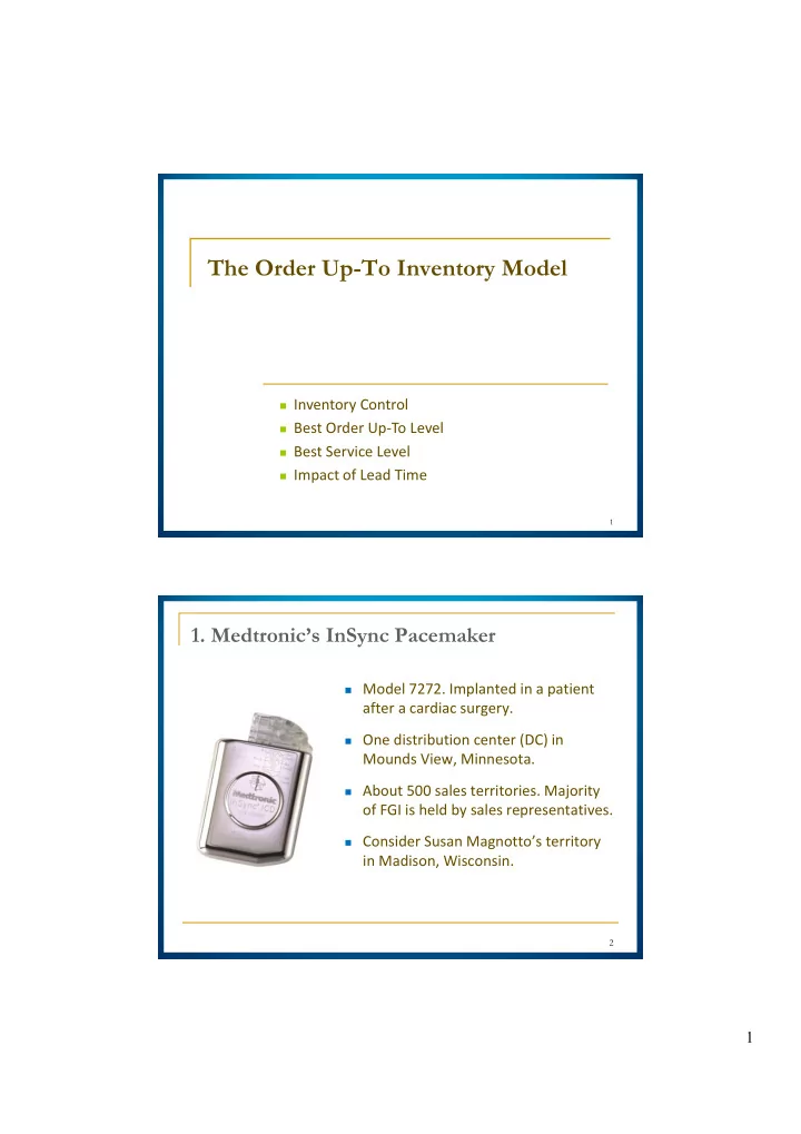
• 1. Medtronic’s InSync Pacemaker

 Model 7272. Implanted in a patient

after a cardiac surgery.

 One distribution center (DC) in

Mounds View, Minnesota.

 About 500 sales territories. Majority

• f FGI is held by sales representatives.

 Consider Susan Magnotto’s territory

in Madison, Wisconsin.

2

2

Demand and Inventory at the DC

• Avg. monthly demand = 349
• Std. Dev. of monthly demand =

122.28

• Avg. weekly demand = 349/4.33 =

80.6 Standard deviation of weekly demand =

(Assume 4.33 weeks per month and independent weekly demands.)

81 . 58 33 . 4 / 38 . 122 

100 200 300 400 500 600 700 Jan Feb Mar Apr May Jun Jul Aug Sep Oct Nov Dec Month Units

Monthly implants (columns) and end

• f month inventory (line)

3

Demand and Inventory in Susan’s Territory

Total annual demand = 75 Average daily demand = 0.29 units (75/260), assuming 5 days per week. Poisson demand distribution works better for slow moving items

2 4 6 8 10 12 14 16 Jan Feb Mar Apr May Jun Jul Aug Sep Oct Nov Dec Month Units

Monthly implants (columns) and end

• f month inventory (line)

4

3

Medtronic’s Inventory Problem

 Patients and surgeons do not tolerate backorders.  The pacemaker is small and has a long shelf life.  Sales incentive system.  Each representative is given a par level which is set quarterly

based on previous sales and anticipated demand. Objective: Because the gross margins are high, Medtronic wants an inventory control policy to minimize inventory investment while maintaining a very high fill rate.

5

Review: Reasons to Hold Inventory

 Pipeline Inventory  Seasonal Inventory  Cycle Inventory  Decoupling Inventory/Buffers  Safety Inventory

6

4

Review: Reasons to Hold Less Inventory

7  Inventory might become obsolete.  Inventory might perish.  Inventory might disappear.  Inventory requires storage space

and other overhead cost.

 Opportunity cost. 8

Review: Inventory Costs

 Holding or Carrying cost

Overestimate the demand

storage cost: facility, handling risk cost: depreciation, pilferage, insurance

• pportunity cost

 Ordering or Setup cost

cost placing an order or changing machine setups

 Shortage costs or Lost Sales

Underestimate the demand

costs of canceling an order or penalty Annual cost ≈ 20% to 40% of the inventory’s worth

5

Review: Inventory Performance

9

 Throughput rate = average daily sales  Throughput time = days of supply  avg. Inventory value = avg. daily sales × avg. throughput time  Days of supply =

average daily sales average inventory value _____________________

Order Receipt On Shelf Sales

Review: Inventory Performance

10  Monthly Inventory turn =  Service level = in‐stock probability before the

replenishment order arrives

 Fill rate =

Cost of Goods Sold in one month _________________________ average inventory value number of demands number of sales _________________

6

11

Review: Multi-Period Inventory Models

Q model: fixed order quantity

R is the reorder point and is based on lead time L and the forecast. Place a new order whenever the inventory level drops to R.

12

Review: P model: fixed time period

T is the review period. S is the target inventory level determined by the forecasts. We place an order to bring the inventory level up to S.

7

 amount of inventory carried in addition to the expected

demand, in order to avoid shortages when demand increases

 depends on service level, demand variability, order lead time  service level depends on Holding cost  Shortage cost 13

Review: Safety Stock

safety stock Service level=probability of no shortage =P (demand ≤ inventory) =P(demand ≤ E(D)+safety stock)

14

Review: Q Models with Safety Stock

d =daily demand d=std dev. of daily demand

d

L z L d       Service level or probability of no shortage =95% (99%)  z=1.64 (2.33)

Timespan=Lead time L (in days)

R=expected demand during L + safety stock

8

15

Review: P Models with Safety Stock

Ex 15.6

Timespan = length of review period + lead time = T + L Order Quantity = target inventory – inventory position

d

L T z L T d        ) (

Target Inventory = expected demand + safety stock

• 2. The Order Up-To Model (P models)

 Time is divided into periods of equal length, e.g., one week.  During a period the following sequence of events occurs:

 A replenishment order can be submitted.  A previous order is received. (lead times = l)  Random demand occurs.

l = 1 Order Receive period 0

• rder

Demand

• ccurs

Order Receive period 1

• rder

Demand

• ccurs

Order Receive period 2

• rder

Demand

• ccurs

Time

Period 1 Period 2 Period 3

16

9

Order Up-To Model Definitions

 On‐order inventory (pipeline inventory) = the number of units

that have been ordered but have not been received.

 On‐hand inventory = number of units physically in stock  Backorder = total amount of demand yet to be satisfied.  Inventory level = On‐hand inventory ‐ Backorder. 實體  Inventory position = On‐order inventory + Inventory level. 帳面  Order up‐to level, S is the maximum inventory position or

target inventory level or base stock level.

17

Order Up-To Model Implementation

Each period’s order quantity = S – Inventory position

 Suppose S = 4.

If begins with an inventory position = 1, order 4 ‐ 1 = 3 If begins with an inventory position = ‐3, order 4 ‐ (‐3) = 7

 S = 4. We begin with an inventory position = 1 and order 3.

If demand were 10 in period 1, then the inventory position at the start of period 2 is 1 – 10 + 3 = ‐6.  order 4 – (‐6)=10 units Pull system: order quantity = the previous period’s demand

18

10

Solving the Order-up-to Model

 Given an order‐up‐to level S  What is the average inventory?  What is the expected lost sale?  What is the best order‐up‐to level? 19

Order Up-To Level and Inventory Level

 On‐order inventory + Inventory level at the beginning of

Period 1 = S

 Inventory level at the end of Period l +1 = S ‐ demand over

recent l +1 periods.

 Ex: S = 6, l = 3, and 2 units on‐hand at the start of period 1

D1 D2 D3 D4 ?

Period 1

Time

Inventory level at the end of period 4 = 6 - D1 – D2 – D3 – D4

Period 2 Period 3 Period 4

20

11

Similarity with a Newsvendor Model

This is like a Newsvendor model in which the order quantity is S and the demand distribution is demand over l +1 periods. S

Period 1 Time

…

…

Period 4

D

S – D > 0, so there is

• n‐hand inventory

S – D < 0, so there are backorders

D = demand

• ver l +1

periods

21

Expected On-Hand Inventory and Backorder

 Expected on‐hand inventory at the end of a period can be

evaluated like Expected left over inventory in the Newsvendor model with Q = S.

 Expected backorder at the end of a period can be evaluated

like Expected lost sales in the Newsvendor model with Q = S.

 Expected on‐order inventory

= Expected demand in a period x lead time

This comes from Little’s Law. Note that it equals the expected demand

• ver l periods, not l +1 periods.

22

12

Key Performance Measures

 The stockout probability is the probability at least one unit is

backordered in a period:

 The in‐stock probability is the probability all demand is filled in

a period:

 The fill rate is the fraction of demand within a period that is

NOT backordered:

Expected backorder Fill rate 1- Expected demand in one period 

       

S periods 1 l

• ver

Demand Prob S periods 1 l

• ver

Demand Prob y probabilit Stockout        1

   

S periods 1 l

• ver

Demand Prob y probabilit Stockout

• 1

y probabilit stock

• In

   

23

Medtronic: Demand over l+1 Periods at DC

DC

 The period length is one week, the replenishment lead time is

three weeks, l = 3

 Assume demand is normally distributed:

 Mean weekly demand is 80.6 (from demand data)  Standard deviation of weekly demand is 58.81  Expected demand over l +1 weeks is (3 + 1) x 80.6 = 322.4  Standard deviation of demand over l +1 weeks is 117.6

6 . 117 81 . 58 1 3   

24

13

DC’s Expected Backorder Assuming S = 625

Expected backorder ≈ Expected lost sales in a Newsvendor model:

 Suppose S = 625 at the DC  Normalize the order up‐to level:  Lookup L(z) in the Standard Normal Loss Function Table:

L(2.57)=0.0016

 Convert expected lost sales, L(z), into the expected

backorder with the actual normal distribution that represents demand over l+1 periods:

57 . 2 6 . 117 4 . 322 625        S z 19 .      0.0016 117.6 L(z) backorder Expected 

25

Other DC Performance Measures

 % of demand is filled immediately (not backorders)  average number of units on‐hand at the end of a period.  There are 241.8 units on‐order at any given time.

0.19 1 1 99.76%. 80.6 Expected backorder Fill rate

• Expected demand in one period

   

 

1 625-322.4 0.19 302.8. Expected on-hand inventory S-Expected demand over l periods Expected backorder =      80.6 3 241.8. Expected on-order inventory Expected demand in one period Lead time =    

26

14

Choose S with Normally Distributed Demand

Suppose the target in‐stock probability at the DC is 99.9%

 From the Standard Normal Distribution Function Table,

(3.08)=0.9990

 So we choose z = 3.08  To convert z into an order up‐to level:  Note that  and  are the parameters of the normal

distribution that describes demand over l + 1 periods.

322.4 3.08 117.6 685 S z         

27

Medtronic: Demand at Susan’s Region

Susan’s territory:

 The period length is one day, the replenishment lead time

is one day, l =1

 Assume demand is Poisson distributed:

 Mean daily demand is 0.29 (from demand data)  Expected demand over l+1 days is 2 x 0.29 = 0.58  Recall, the Poisson is completely defined by its mean

(standard deviation is the square root of the mean)

28

15

Using EXCEL to Calculate the Poisson Loss

Mean=0.58 Suppose S = 3 Expected backorder L(S)= 0.00335 Stock out probability = 0.0029

Poisson Mean 0.58 Order Size 3 demand lost sales probability expected loss 0.5599 0.0000 1 0.3247 0.0000 2 0.0942 0.0000 3 0.0182 0.0000 4 1 0.0026 0.0026 5 2 0.0003 0.0006 6 3 0.0000 0.0001 7 4 0.0000 0.0000 8 5 0.0000 0.0000 9 6 0.0000 0.0000 10 7 0.0000 0.0000 expected lost sales= 0.00335

29

Performance Measures in Susan’s Territory

 Order‐up‐to level S = 3

 Expected backorder= L(S)= 0.00335  In‐stock = 99.70%  Fill rate = 1 – 0.00335 / 0.29 = 98.84%  Expected on‐hand = S – demand over l+1 periods +

backorder = 3 – 0.58 + 0.00335 = 2.42

 Expected on‐order inventory = Demand over the lead time

= 0.29

30

16

Choose S with Poisson Demand

 Period length is 1 day, replenishment lead time is l = 1  Demand over l + 1 days is Poisson with mean 0.58  Target in‐stock is 99.9%  In Susan’s territory, S = 4 is the smallest value that meets the

target in‐stock probability:

S Probability { Demand over l+1 periods <= S ) 0.5599 1 0.8846 2 0.9788 3 0.9970 4 0.9997 5 1.0000

31

Best Order-up-to Level via Cost Minimization

 If S is too high, there are holding costs, Co = 0.000337p  If S is too low, there are lost sales, Cu = 0.75p  Best order up‐to level must satisfies  Optimal in‐stock probability is 99.96% because

32

17

14.8 Impact of Period Length on DC Cost

 Increasing the period length leads to larger and less

frequent orders:

33

200 400 600 800 1000 1200 1400 1600 2 4 6 8 10 12 14 16 200 400 600 800 1000 1200 1400 1600 2 4 6 8 10 12 14 16 200 400 600 800 1000 1200 1400 1600 2 4 6 8 10 12 14 16 200 400 600 800 1000 1200 1400 1600 2 4 6 8 10 12 14 16

2000 4000 6000 8000 10000 12000 14000 16000 18000 20000 22000 1 2 3 4 5 6 7 8 9 Period length (in weeks) Cost

Inventory Holding Costs vs. Ordering Costs

478 5 . 12 5200 275 2 2        h R K Q



Costs:

 Ordering costs = $275 per order  Holding costs = 25% per year  Unit cost = $50  Holding cost per unit per year =

25% x $50 = 12.5



Period length of 4 weeks minimizes costs:

 This implies the average order

quantity is 4 x 100 = 400 units



EOQ model:

Ordering costs Inventory holding costs Total costs 34

18

20 40 60 80 100 120 140 90% 91% 92% 93% 94% 95% 96% 97% 98% 99% 100% Fill rate Expected inventory Increasing standard deviation

14.9 Better Service Requires More Inventory

More inventory is needed as demand uncertainty increases for any fixed fill rate. The required inventory is more sensitive to the fill rate level as demand uncertainty increases

35

Shorten Lead Times Reduce Inventory

Reducing the lead time reduces expected inventory, especially as the target fill rate increases

100 200 300 400 500 600 5 10 15 20 Lead time Expected inventory

The impact of lead time on expected inventory for four fill rate targets, 99.9%, 99.5%, 99.0% and 98%, top curve to bottom curve respectively.

36

19

Do Not Forget About Pipeline Inventory

500 1000 1500 2000 2500 3000 5 10 15 20 Lead time Inventory

Reducing the lead time reduces expected inventory and pipeline inventory The impact on pipeline inventory can be even more dramatic that the impact on expected inventory

expected inventory + pipeline inventory expected inventory

37  The higher the order up‐to level, the better the service.  Key factors that determine the amount of inventory needed

• The length of the replenishment lead time.
• The desired service level (fill rate or in‐stock probability).
• Demand uncertainty.

 When inventory obsolescence is not an issue, the optimal

service level is generally quite high.

38