Chapter 9 Managing Inventory Types of Inventory ABC Analysis Q - PDF document

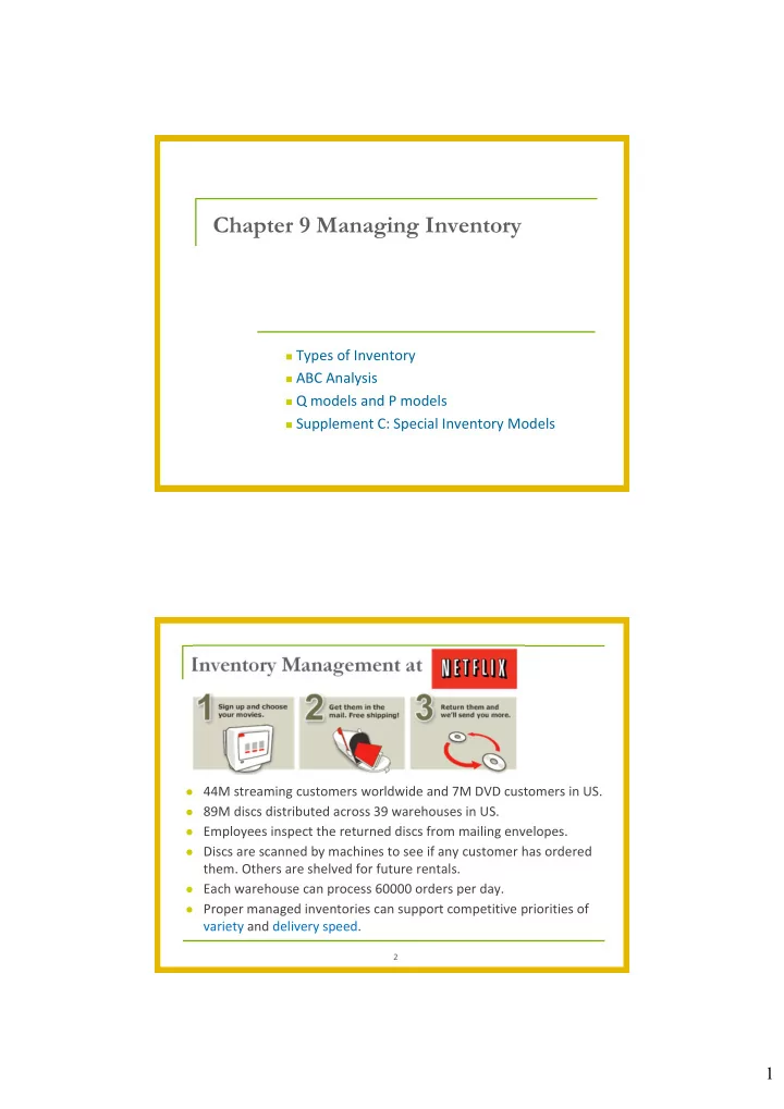
Chapter 9 Managing Inventory  Types of Inventory  ABC Analysis  Q models and P models  Supplement C: Special Inventory Models Inventory Management at  44M streaming customers worldwide and 7M DVD customers in US.  89M discs distributed across 39 warehouses in US.  Employees inspect the returned discs from mailing envelopes.  Discs are scanned by machines to see if any customer has ordered them. Others are shelved for future rentals.  Each warehouse can process 60000 orders per day.  Proper managed inventories can support competitive priorities of variety and delivery speed. 2 1

What is Inventory? A stock of materials used to satisfy customer demand or to support the production of services or goods. Manufacturing Inventory raw materials, WIP, maintenance and repairs, supplies, FGI Retail Inventory merchandise, supplies, goods in transit (pipeline inventory) What is a Inventory Management? The planning and controlling of inventories to meet the competitive priorities of the organization. 4 Pressures for Small Inventories Inventory holding cost  Cost of capital (opportunity cost)  Storage and handling costs: space, labor, machines  Taxes  Insurance  Shrinkage  Pilferage by customers or employees  Obsolescence due to model changes or new products  Deterioration: limited shelf life 5 2

Pressures for Large Inventories  Customer service: stockout or backorder  Ordering cost: fixed cost of preparing a purchase order  Setup cost: fixed cost of changing over a machine to produce a different product.  Labor and equipment utilization  Transportation cost: full truckload or full container  Payments to suppliers (quantity discount) 6 Inventory Costs  Purchase Cost  Holding or Carrying cost order too much or too early opportunity cost 資金積壓的潛在損失 storage cost 倉儲設備、進出盤點 shrinkage cost 貶值、偷竊、毀損、保費 Ordering or Setup cost 前置作業成本 order too often or too little 對外採購：聯繫、運輸、驗收 內部製造：停機調整、試產  Shortage costs or Lost Sales order too little or too late 停工減產的損失、延誤交貨的罰款 銷售減少的利潤損失 7 3

Types of Inventory  Cycle Inventory : Inventory that varies between orders.  Safety Stock Inventory : surplus inventory that protects against uncertainties in demand, lead time, and supply changes.  Anticipation Inventory : used to absorb uneven rates of demand or supply. (price increase)  Pipeline Inventory 在途庫存 : inventory in transit between two stocking points. 8 Cycle Inventory The lot size, Q , varies directly with the elapsed time (or cycle) between orders. The longer the time between orders for a given item, the greater the cycle inventory must be. Q + 0 Q Average cycle inventory = = 2 2 Pipeline Inventory Average demand per period = d Number of periods in the item’s lead time = L (fixed) Average Pipeline inventory = d L 9 4

Inventory Reduction Tactics 1/2  Cycle inventory: Reduce the lot size  Reduce ordering and setup costs and allow Q to be reduced  Increase repeatability to eliminate the need for changeovers  Safety stock inventory: Place orders closer to the time when they must be received  Improve demand forecasts  Cut lead times  Reduce supply uncertainties  Rely more on equipment and labor buffers 10 Inventory Reduction Tactics 2/2  Anticipation inventory: Match demand rate with production rates  Add new products with different demand cycles  Provide off‐season promotional campaigns  Offer seasonal pricing plans  Pipeline inventory: Reduce lead times  Find more responsive suppliers and select new carriers  Change Q in those cases where the lead time depends on the lot size 11 5

Economic Order Quantity  The lot size, Q , that minimizes total annual inventory holding and ordering costs. Five assumptions: 1. Demand rate is constant and known with certainty. 2. No constraints are placed on the size of each lot. 3. The only two relevant costs are the inventory holding cost and the fixed cost per lot for ordering or setup. 4. Decisions for one item can be made independently of decisions for other items. The lead time is constant and known with certainty. 5.  Use the EOQ 經濟訂貨量 Make‐to‐stock strategy with relatively stable demand.  Carrying and setup costs are known and relatively stable  12 Receive Inventory depletion order (demand rate) How Many to Q On-hand inventory Order? Q Average cycle 2 inventory Time 1 cycle Q 1 Q 1 2 13 6

Calculating EOQ  Annual Demand = D  Annual holding cost Q  = (Average cycle inventory)  (Unit holding cost) = H 2  Annual ordering cost D  =(Number of orders/Year)  (Ordering or setup costs) = S Q Q D    C ( Q ) H 1 S Total costs = 2 Q d 2 DS EOQ *     C 0 EOQ Q Time Between Orders = D dQ H 14 Calculating EOQ Total cost Annual cost (dollars) Holding cost Ordering cost Lot Size ( Q ) 15 7

Example 9.2: Bird Feeder  Sales are 18 units per week, the supplier charges $60 per unit.  Ordering cost is $45.  Annual holding cost is 25 percent of a feeder’s value.  What is the annual cycle‐inventory cost of the current policy of using a 390‐unit lot size? Would a lost size of 468 be better? D =(18 units/week)(52 weeks/year) = 936 units H =0.25($60/unit) = $15 S =$45 Q D 390 936    C ( Q ) H 1 S = ($15) + ($45) 2 390 2 Q = $2,925 + $108 = $3,033 16 Example 9.3 EOQ for bird feeders 2 DS 2 ( 936 ) 45   = 74.94 or 75 units EOQ H 15 17 8

Managerial Insights from the EOQ SENSITIVITY ANALYSIS OF THE EOQ Parameter EOQ Parameter EOQ Comments Change Change 2 DS Increase in lot size is in proportion Demand ↑ ↑ to the square root of D . H 2 DS Order/ Weeks of supply decreases and Setup ↓ ↓ inventory turnover increases H Costs because the lot size decreases. 2 DS Holding Larger lots are justified when ↓ ↑ Costs holding costs decrease. H 18 Inventory Control Systems Periodic Review System Continuous Review System Fixed Order Period Fixed Order Quantity P model Q model 19 9

Continuous Review System  Q model or fixed order quantity system  Tracks inventory position (IP)  Reorder point system (ROP) and fixed order quantity (Q)  Decision Includes scheduled receipts (SR), on‐hand inventory (OH), and back orders (BO) Inventory position = On‐hand inventory + Scheduled receipts – Backorders IP = OH + SR – BO Rule: If IP  ROP, place an order of size Q 20 Continuous Review System IP Order Order Order received received received On-hand inventory Q Q Q OH R Order Order Order placed placed placed L L L Time TBO TBO TBO Selecting the Reorder Point depends on Demand and Lead Times. 21 10

Example 9.4 Demand for chicken soup at a supermarket is always 25 cases a day and the lead time is always 4 days. The on‐hand inventory has only 10 cases. No backorders currently exist, but there is one open order in the pipeline for 200 cases. Should a new order be placed? R = Total demand during lead time = (25)(4) = 100 cases IP = OH + SR – BO= 10 + 200 – 0 = 210 cases 22 Continuous Review System 2: Variable Demand IP IP IP Order Order received received Order received On-hand inventory Q Q Q R Order Order Order placed placed placed 0 Time L 1 L 2 L 3 TBO 1 TBO 2 TBO 3 Select ROP base on Demand, Lead Times, and Safety Stock. 23 11

Example 9.5  A distribution center receives its inventory from a mega warehouse with a lead time ( L ) of 5 days. The DC uses a reorder point ( R ) of 300 sets and a fixed order quantity ( Q ) of 250 sets. Current on‐hand inventory at the end of Day 1 is 400 sets. There are no scheduled receipts (SR) and no backorders (BO). All demands and receipts occur at the end of the day .  Determine when to order using a Q system 24 Example 9.5 ROP=300, Q=250, L=5 days Day Demand OH SR BO IP Q 400 + 0 = 400 1 400 60 340 340 + 0 = 340 2 260 < R before ordering 250 due 250 after ordering 3 80 260 260+250=510 after ordering Day 8 40 220 250 220 + 250 = 470 4 145 + 250 = 395 75 145 250 5 55 90 250 90 + 250 = 340 6 95 0 250+ 250 = 500 5 0+250–5=245< R before ordering 245 + 250 = 495 after ordering 250 due 7 after ordering Day 12 250‐50‐5 50 195 + 250 = 445 8 250 =195 25 12

Continuous Review System 2: Reorder Point  Assume variable demand and constant lead time Reorder point = Average demand during lead time + Safety stock = dL + Safety stock = dL + z  σ dLT  Choosing a Reorder Point 2. Determine the distribution of demand during lead time 1. Choose an appropriate service‐level policy 3. Use the formula to calculate the safety stock and reorder point levels 26 Distribution of Demand during Lead Time  Specify mean and standard deviation of daily demand σ d d  Standard deviation of demand during lead time σ dLT = σ d 2 L = σ d L σ dlt = 25.98 σ d = 15 σ d = 15 σ d = 15 + = + 75 75 75 225 Demand for Demand for Demand for Demand for 3-week week 1 week 2 week 3 lead time 27 13