
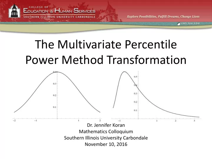
SLIDE 1
The Multivariate Percentile Power Method Transformation
- Dr. Jennifer Koran
Mathematics Colloquium Southern Illinois University Carbondale November 10, 2016
The Multivariate Percentile Power Method Transformation Dr. - - PowerPoint PPT Presentation
The Multivariate Percentile Power Method Transformation Dr. Jennifer Koran Mathematics Colloquium Southern Illinois University Carbondale November 10, 2016 Power Method (PM) Transformation Headrick (2010): 1
Mathematics Colloquium Southern Illinois University Carbondale November 10, 2016
𝑛 𝑗=1
𝑎 𝑨 = 𝜒 𝑨 = 2𝜌 −1
2 exp − 𝑨2 2
𝑨 −∞
2 + 2𝑑3 2 + 6𝑑2𝑑4 + 15𝑑4 2
3 + 6𝑑2 2𝑑3 + 72𝑑2𝑑3𝑑4 + 270𝑑3𝑑4 2
4 + 60𝑑2 2𝑑3 2 + 60𝑑3 4 + 60𝑑2 3𝑑4 + 936𝑑2𝑑3 2𝑑4
2𝑑4 2 + 4500𝑑3 2𝑑4 2 + 3780𝑑2𝑑4 3
4 − 3.
𝜄0.50−𝜄0.10 𝜄0.90−𝜄0.50
𝜄0.75−𝜄0.25 𝛿2
3
2
3
3
3
3
3
3
2
3
3
𝑑1 = 𝛿1 𝑑2 = 𝛿2 𝛿4𝑨0.90
3
− 𝑨0.75
3
2𝑨0.90
3
𝑨0.75 − 2𝑨0.90𝑨0.75
3
𝑑3 = 𝛿2 1 − 𝛿3 2 1 + 𝛿3 𝑨0.90
2
𝑑4 = − 𝛿2 𝛿4𝑨0.90 − 𝑨0.75 2𝑨0.90
3
𝑨0.75 − 2𝑨0.90𝑨0.75
3
𝑞 𝑎 =
𝑗=1 𝑛
𝑑𝑗𝑎𝑗−1
Vale and Maurelli (1983) 𝜍𝑘𝑙 = 𝐹 𝑞 𝑎
𝑘 𝑞 𝑎𝑙
= 𝑠
𝑘𝑙 𝑑 𝑘2𝑑𝑙2 + 3𝑑 𝑘4𝑑𝑙2 + 3𝑑 𝑘2𝑑𝑙4 + 9𝑑 𝑘4𝑑𝑙4 + 2𝑑 𝑘1𝑑𝑙1𝑠 𝑘𝑙 + 6𝑑 𝑘4𝑑𝑙4𝑠 𝑘𝑙 2
Specified Correlation Matrix Ρ 1 2 3 4 1 1 2 0.80 1 3 0.70 0.60 1 4 0.65 0.50 0.45 1 Intermediate Correlation Matrix
𝑆
1 2 3 4 1 1 2 0.897 1 3 0.831 0.666 1 4 0.750 0.580 0.489 1
𝑘𝑙
𝑘𝑙
Specified Correlation Matrix Ξ 1 2 3 4 1 1 2 0.80 1 3 0.70 0.60 1 4 0.65 0.50 0.45 1 Intermediate Correlation Matrix, n = 25 𝑆 1 2 3 4 1 1 2 0.835 1 3 0.739 0.639 1 4 0.689 0.536 0.484 1
Figure 1. The power method (PM) pdf of Distribution 1. Conventional PM Percentile PM Percentiles Skew: 𝛽3 = 0 Kurtosis: 𝛽4 = 25 𝑑1 = 0 𝑑2 = 0.2553 𝑑3 = 0 𝑑4 = 0.2038 Left-right tail-weight ratio: 𝛿3 = 1.0000 Tail-weight factor : 𝛿4 = 0.3105 𝑑1 = 0 𝑑2 = 0.4327 𝑑3 = 0 𝑑4 = 0.3454
𝜄 𝑦 0.10 = −0.7560 𝜄 𝑦 0.25 = −0.2347 𝜄 𝑦 0.50 = 0 𝜄 𝑦 0.75 = 0.2347 𝜄 𝑦 0.90 = 0.7560
Figure 2. The power method (PM) pdf of Distribution 2. Conventional PM Percentile PM Percentiles Skew: 𝛽3 = 3 Kurtosis: 𝛽4 = 21 𝑑1 = −0.2523 𝑑2 = 0.4186 𝑑3 = 0.2523 𝑑4 = 0.1476 Left-right tail-weight ratio: 𝛿3 = 0.3130 Tail-weight factor : 𝛿4 = 0.3335 𝑑1 = −0.3203 𝑑2 = 0.5315 𝑑3 = 0.3203 𝑑4 = 0.1874
𝜄 𝑦 0.10 = −0.6851 𝜄 𝑦 0.25 = −4652 𝜄 𝑦 0.50 = −0.2523 𝜄 𝑦 0.75 = 0.1901 𝜄 𝑦 0.90 = 1.0092
Figure 3. The power method (PM) pdf of Distribution 3. Conventional PM Percentile PM Percentiles Skew: 𝛽3 = 2 Kurtosis: 𝛽4 = 7 𝑑1 = −0.2600 𝑑2 = 0.7616 𝑑3 = 0.2600 𝑑4 = 0.0531 Left-right tail-weight ratio: 𝛿3 = 0.2841 Tail-weight factor : 𝛿4 = 0.1894 𝑑1 = −0.2908 𝑑2 = 0.8516 𝑑3 = 0.2908 𝑑4 = 0.0593
𝜄 𝑦 0.10 = −0.9207 𝜄 𝑦 0.25 = −0.6717 𝜄 𝑦 0.50 = −0.2600 𝜄 𝑦 0.75 = 0.3882 𝜄 𝑦 0.90 = 1.2547
Figure 4. The power method (PM) pdf of Distribution 4. Conventional PM Percentile PM Percentiles Skew: 𝛽3 = 0 Kurtosis: 𝛽4 = 0 𝑑1 = 0 𝑑2 = 1 𝑑3 = 0 𝑑4 = 0 Left-right tail-weight ratio: 𝛿3 = 0.0000 Tail-weight factor : 𝛿4 = 0.1226 𝑑1 = 0 𝑑2 = 1 𝑑3 = 0 𝑑4 = 0
𝜄 𝑦 0.10 = −1.2816 𝜄 𝑦 0.25 = −0.6745 𝜄 𝑦 0.50 = 0 𝜄 𝑦 0.75 = 0.6745 𝜄 𝑦 0.90 = 1.2816
Skew (𝛽3) and Kurtosis (𝛽4) results for the Conventional PM. Dist Parameter Estimate 95% Bootstrap C.I. Standard Error Relative Bias % 1 𝛽3 = 0
0.013660
4.4560 4.4011,4.5261 0.030200
2 𝛽3 = 3 1.5750 1.5579,1.5911 0.008122
𝛽4 = 21 3.6960 3.6452,3.7525 0.027010
3 𝛽3 = 2 1.2780 1.2677,1.2893 0.005561
𝛽4 = 7 1.5230 1.4849,1.5662 0.020430
4 𝛽3 = 0 0.0034
0.003626
0.005579
Dist Parameter Estimate 95% Bootstrap C.I.
Relative Bias % 1 𝛿3 = 1.0000 1.0050 0.9942, 1.0154 0.005348
0.3208 0.3191, 0.3227 0.000947
𝛿3 = 0.3430 0.3466 0.3438, 0.3497 0.001485 1.04 𝛿4 = 0.3868 0.3972 0.3954, 0.3993 0.000983 2.70 3 𝛿3 = 0.4361 0.4472 0.4444, 0.4501 0.001464 2.53 𝛿4 = 0.4872 0.4960 0.4943, 0.4980 0.001003 1.80 4 𝛿3 = 1.0000 0.9978 0.9912, 1.0045 0.003380
0.5294 0.5279, 0.5310 0.000801
Correlation results for the Conventional PM, 𝑜 = 25
Parameter Estimate 95% Bootstrap C.I. Standard Error RSE Relative Bias % 𝜍12
∗ = 0.80
0.8275 0.8258 , 0.8290 0.002612 0.0032 3.43 𝜍13
∗ = 0.70
0.7358 0.7340 , 0.7376 0.001944 0.0026 5.12 𝜍14
∗ = 0.65
0.6959 0.6943 , 0.6976 0.001575 0.0023 7.07 𝜍23
∗ = 0.60
0.6209 0.6185 , 0.6236 0.002075 0.0033 3.48 𝜍24
∗ = 0.50
0.5376 0.5354 , 0.5400 0.001595 0.0030 7.52 𝜍34
∗ = 0.45
0.4677 0.4650 , 0.4700 0.001638 0.0035 3.93
Correlation results for the Percentiles PM, 𝑜 = 25
Parameter Estimate 95% Bootstrap C.I. Standard Error RSE Relative Bias % 𝜊12 = 0.80 0.8141 0.8123 , 0.8146 0.002007 0.0025 1.76 𝜊13 = 0.70 0.7138 0.7119 , 0.7162 0.002005 0.0028 1.97 𝜊14 = 0.65 0.6658 0.6646 , 0.6685 0.001954 0.0029 2.43 𝜊23 = 0.60 0.6142 0.6115 , 0.6154 0.001719 0.0028 2.37 𝜊24 = 0.50 0.5154 0.5131 , 0.5177 0.001809 0.0035 3.09 𝜊34 = 0.45 0.4646 0.4631 , 0.4685 0.001534 0.0033 3.23
Skew (𝛽3) and Kurtosis (𝛽4) results for the Conventional PM. Dist Parameter Estimate 95% Bootstrap C.I. Standard Error Relative Bias % 1 𝛽3 = 0 2.562 2.5383, 2.5823 0.01117
𝛽4 = 25 22.15 21.6873, 22.6698 0.24850
2 𝛽3 = 3 2.180 2.1668, 2.1944 0.00697
𝛽4 = 21 13.36 13.0936, 13.6467 0.14100
3 𝛽3 = 2
0.01100
18.57 18.2203, 18.9412 0.18330
4 𝛽3 = 0 1.54 1.5246, 1.5539 0.00743
𝛽4 = 0 12.91 12.6537, 13.1903 0.13610
Left-right tail-weight ratio 𝛿3 and tail-weight factor 𝛿4 results for Percentiles PM. Dist Parameter Estimate 95% Bootstrap C.I.
Relative Bias % 1 𝛿3 = 1.0000 1.0000 0.9978, 1.0020 0.001062
0.3108 0.3105, 0.3112 0.000171 0.11 2 𝛿3 = 0.3430 0.3432 0.3426, 0.3438 0.000308
0.3873 0.3869, 0.3877 0.000203 0.14 3 𝛿3 = 0.4361 0.4359 0.4353, 0.4364 0.000287
0.4874 0.4870, 0.4877 0.000189
𝛿3 = 1.0000 1.0000 0.9991, 1.0014 0.000539
0.5264 0.5261, 0.5267 0.000159
Correlation results for the Conventional PM, 𝑜 = 750
Parameter Estimate 95% Bootstrap C.I. Standard Error RSE Relative Bias % 𝜍12
∗ = 0.80
0.8012 0.8009 , 0.8018 0.000622 0.0008 0.15 𝜍13
∗ = 0.70
0.7037 0.7033 , 0.7042 0.000496 0.0007 0.53 𝜍14
∗ = 0.65
0.6546 0.6542 , 0.6549 0.000330 0.0005 0.71 𝜍23
∗ = 0.60
0.6007 0.6001 , 0.6012 0.000464 0.0008 0.11 𝜍24
∗ = 0.50
0.5022 0.5018 , 0.5026 0.000266 0.0005 0.45 𝜍34
∗ = 0.45
0.4506 0.4501 , 0.4510 0.000271 0.0006 0.12
Correlation results for the Percentiles PM, 𝑜 = 750
Parameter Estimate 95% Bootstrap C.I. Standard Error RSE Relative Bias % 𝜊12 = 0.80 0.8001 0.8001 , 0.8005 0.000338 0.0004 0.02 𝜊13 = 0.70 0.7004 0.7000 , 0.7007 0.000322 0.0005 0.05 𝜊14 = 0.65 0.6502 0.6499 , 0.6506 0.000303 0.0005
0.6002 0.5999 , 0.6006 0.000302 0.0005
0.5000 0.4995 , 0.5005 0.000328 0.0007
0.4502 0.4497 , 0.4506 0.000293 0.0007
𝑘 𝑞 𝑎𝑙
𝑘 𝑞 𝑎𝑙
𝑘1 𝑑𝑙1 + 𝑑𝑙3 + 𝑑𝑙3 𝑑𝑙1 + 𝑑𝑙3
𝑘𝑙 𝑑 𝑘2𝑑𝑙2 + 3𝑑 𝑘4𝑑𝑙2 + 3𝑑 𝑘2𝑑𝑙4 + 9𝑑 𝑘4𝑑𝑙4
𝑘𝑙 2 2𝑑 𝑘3𝑑𝑙3 + 𝑠 𝑘𝑙 3 6𝑑 𝑘4𝑑𝑙4
𝑘1 + 𝑑 𝑘3 and 𝑤𝑘 = 𝑑 𝑘2 2 + 2𝑑 𝑘3 3 + 6𝑑 𝑘2𝑑 𝑘4 + 15𝑑 𝑘4 2
Macro call:
Percentiles File (ex2percentiles.txt):
Correlations File (ex2correlations.txt):
Fleishman, A. I. (1978). A method for simulating non-normal distributions. Psychometrika, 43, 521-532. doi: 10.1007/BF02293811 Headrick, T. C. (2010). Statistical simulation: power method polynomials and other
Karian, Z. A., & Dudewicz, E. J. (2011). Handbook of fitting statistical distributions with R. Boca Raton FL: CRC Press. Koran, J., & Headrick, T.C. (2016). A percentile-based power method in SAS: Simulating multivariate non-normal continuous distributions. Journal of Modern Applied Statistical Methods, 15(1). Available from http://digitalcommons.wayne.edu/jmasm/vol15/iss1/42 Koran, J., Headrick, T.C., & Kuo,T.-C. (2015). Simulating univariate and multivariate nonnormal distributions through the method of percentiles. Multivariate Behavioral Research, 50, 216-232. doi: 10.1080/00273171.2014.963194 Vale, C. D., & Maurelli, V. A. (1983). Simulating multivariate nonnormal distributions. Psychometrika, 48, 465-471. doi: 10.1007/BF02293687