Outline Multivariate Data 1 Multivariate Parametric Methods - PowerPoint PPT Presentation

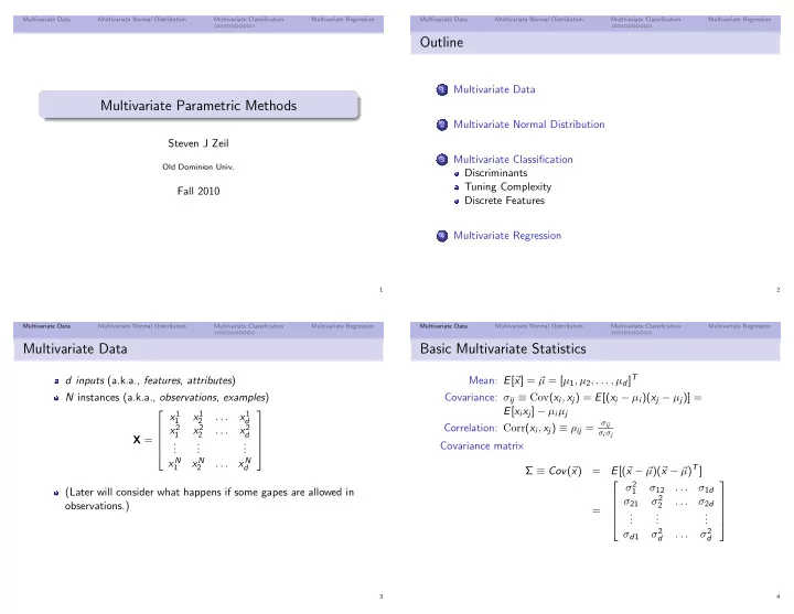
Multivariate Data Multivariate Normal Distribution Multivariate Classification Multivariate Regression Multivariate Data Multivariate Normal Distribution Multivariate Classification Multivariate Regression Outline Multivariate Data 1 Multivariate Parametric Methods Multivariate Normal Distribution 2 Steven J Zeil Multivariate Classification 3 Old Dominion Univ. Discriminants Tuning Complexity Fall 2010 Discrete Features Multivariate Regression 4 1 2 Multivariate Data Multivariate Normal Distribution Multivariate Classification Multivariate Regression Multivariate Data Multivariate Normal Distribution Multivariate Classification Multivariate Regression Multivariate Data Basic Multivariate Statistics µ = [ µ 1 , µ 2 , . . . , µ d ] T d inputs (a.k.a., features , attributes ) Mean: E [ � x ] = � N instances (a.k.a., observations , examples ) Covariance: σ ij ≡ Cov ( x i , x j ) = E [( x i − µ i )( x j − µ j )] = E [ x i x j ] − µ i µ j  x 1 x 1 x 1  . . . 1 2 d σ ij Correlation: Corr ( x i , x j ) ≡ ρ ij = x 2 x 2 x 2 . . . σ i σ j  1 2  d X = . . .   . . . Covariance matrix   . . .   x N x N x N . . . 1 2 d µ ) T ] Σ ≡ Cov ( � x ) = E [( � x − � µ )( � x − � σ 2   σ 12 . . . σ 1 d (Later will consider what happens if some gapes are allowed in 1 σ 2 σ 21 . . . σ 2 d observations.)   2 =  . . .  . . .   . . .   σ 2 σ 2 σ d 1 . . . d d 3 4

Multivariate Data Multivariate Normal Distribution Multivariate Classification Multivariate Regression Multivariate Data Multivariate Normal Distribution Multivariate Classification Multivariate Regression Multivariate Parameter Estimation Imputation � N t =1 x t What if certain instances have missing attributes? Sample Mean � m : m i = , i = 1 . . . d i N Throw out entire instance? � N t =1 ( x t i − m i )( x t j − m j ) Covariance Matrix: s ij = problem if the sample is small N s ij Correlation Matrix: R : r ij = Imputation : fill in the missing value s i s j Mean imputation: use the expected value Imputation by regression: predict based on other attributes 5 6 Multivariate Data Multivariate Normal Distribution Multivariate Classification Multivariate Regression Multivariate Data Multivariate Normal Distribution Multivariate Classification Multivariate Regression Multivariate Normal Distribution Slicing Any slice (projection) along a single direction � w is normal: � x ∼ N d ( � µ, Σ) w T � w T � w T Σ � � x ∼ N ( � µ, � w ) 1 � − 1 � µ ) T Σ − 1 ( � x − � x − � p ( � x ) = (2 π ) d / 2 | Σ | 1 / 2 exp 2( � µ ) Any projection onto a linearly transformed set of axes of dimention ≤ d is MV Normal 7 8

Multivariate Data Multivariate Normal Distribution Multivariate Classification Multivariate Regression Multivariate Data Multivariate Normal Distribution Multivariate Classification Multivariate Regression Effects of Covariance Normalized Distance z = x − µ can be seen as a distance from µ to x in normalized σ σ -size units. Generalizing to d dimensions gives the Mahalanobis distance µ ) T Σ − 1 ( � ( � x − � x − � µ ) If x i has larger variance than x j , x i gets lower weight in this distance. If x i and x j are highly correlated, they get less weight than two less correlated variables. A small | Σ | indicates that the samples are close to � µ and/or the variables are highly correlated If | Σ | is zero, then some of the variables are constant or there is a linear dependency among variables. Either way, reduce the dimensionality by removing unneeded variables 9 10 Multivariate Data Multivariate Normal Distribution Multivariate Classification Multivariate Regression Multivariate Data Multivariate Normal Distribution Multivariate Classification Multivariate Regression Special Cases of Mahalanobis Distance Outline µ ) T Σ − 1 ( � d ( � x ) = ( � x − � x − � µ ) Multivariate Data 1 If the x i are independent, off-diagonal elements of Σ are zero Multivariate Normal Distribution 2 d � 2 � x i − µ i � d ( � x ) = Multivariate Classification 3 Σ i Discriminants i =0 Tuning Complexity If the variances are also equal, reduces to Euclidean distance Discrete Features Multivariate Regression 4 11 12

Multivariate Data Multivariate Normal Distribution Multivariate Classification Multivariate Regression Multivariate Data Multivariate Normal Distribution Multivariate Classification Multivariate Regression Multivariate Classification Quadratic Discriminant If p ( � x | C i ) ∼ N ( � µ i , Σ i ), d 2 log 2 π − 1 2 log | S i | − 1 1 � − 1 � m i ) T S − 1 m i ) + log ˆ µ i ) T Σ − 1 g i ( � 2( � x − � ( � x = � x ) = P ( C i ) p ( � x | C i ) = (2 π ) d / 2 | Σ i | 1 / 2 exp 2( � x − � ( � x − � µ i ) i i − 1 2 log | S i | − 1 m i ) T S − 1 m i ) + log ˆ ≃ 2( � x − � ( � x = � P ( C i ) Discriminants are i − 1 2 log | S i | − 1 � � x T S − 1 x T S − 1 m T i S − 1 = � x − 2 � � m i + � � � g i ( � log p ( � x | C i ) + log P ( C i ) m i x ) = i i i 2 2 log 2 π − 1 d 2 log | Σ i | − 1 + log ˆ µ i ) T Σ − 1 P ( C i ) 2( � x − � ( � x − � = µ i ) i x T W i � w T x + w 0 = � x + � i � + log P ( C i ) i This is a quadratic in � x . Estimate as x ) = d 2 log 2 π − 1 2 log | S i |− 1 m i )+log ˆ m i ) T S − 1 g i ( � 2( � x − � ( � x − � P ( C i ) i 13 14 Multivariate Data Multivariate Normal Distribution Multivariate Classification Multivariate Regression Multivariate Data Multivariate Normal Distribution Multivariate Classification Multivariate Regression Simplification: Shared covariance Share a common sample covariance S � ˆ S = P ( C i ) S i i Discriminant simplifies to x ) = 1 likelihoods m i ) T S − 1 ( � m i ) + log ˆ g i ( � 2( � x − � x − � P ( C i ) Although this function is quadratic in � x , it yields a linear x t � discriminant because the � x quadratic term is identical across all i . posterior for C i 15 16

Multivariate Data Multivariate Normal Distribution Multivariate Classification Multivariate Regression Multivariate Data Multivariate Normal Distribution Multivariate Classification Multivariate Regression Linear Discriminant Further Simplification: Independence If we share a common sample covariance S and the variables are independent, then the off-diagonal elements of S are zero. Discriminant simplifies to � 2 d � x t j − m ij x ) = 1 � + log ˆ g i ( � P ( C i ) 2 s j j =1 This is the Naive Bayes Classifier . Each variable is an independent Gaussian Distance measured in standard deviation units 17 18 Multivariate Data Multivariate Normal Distribution Multivariate Classification Multivariate Regression Multivariate Data Multivariate Normal Distribution Multivariate Classification Multivariate Regression Diagonal S Further Simplification: Equal Variances If variances are also equal, Discriminant simplifies to � 2 d � x t j − m ij x ) = 1 � + log ˆ g i ( � P ( C i ) 2 s j =1 This is the nearest mean classifier . 19 20 Ellipsoids are aligned with axes.

Multivariate Data Multivariate Normal Distribution Multivariate Classification Multivariate Regression Multivariate Data Multivariate Normal Distribution Multivariate Classification Multivariate Regression Model Selection Binary Features x j ∈ { 0 , 1 } Assumption Covariance matrix # Parameters p ij = p ( x j = 1 | C i ) S i = S = s 2 I Equal variances 1 If the x j are independent (Naive Bayes) Independent S i = S , s ij = 0 d Shared Covariance S i = S d ( d + 1) / 2 d Different Covariances Kd ( d + 1) / 2 p x j S i � ij (1 − p ij ) (1 − x j ) x | C i ) = p ( � j = i The discriminant in linear � p ij )] + log ˆ g i ( � p ij + (1 − x j ) log (1 − ˆ x ) = [ x j log ˆ P ( C i ) j 21 22 Multivariate Data Multivariate Normal Distribution Multivariate Classification Multivariate Regression Multivariate Data Multivariate Normal Distribution Multivariate Classification Multivariate Regression Discrete Features Multivariate Regression x j ∈ { v 1 , v 2 , . . . , v n j } r t = g ( � x t | w 0 , w 1 , . . . , w d ) + ε p ijk = p ( z jk = 1 | C i ) = p ( x j = v k | C i ) If the x j are independent Multivariate linear model w 0 + w 1 x t 1 + w 2 x t 2 + . . . + w d x t n j d d p z jk � � x | C i ) = p ( � Error: ijk j = i w |X ) = 1 k = i r t − ( w 0 + w 1 x t � 1 + w 2 x t 2 + . . . + w d x t � � E ( � d ) 2 t � � p ijk + log ˆ g i ( � x ) = z jk log ˆ P ( C i ) x 1 x 1 x 1 r 1     1 . . . j k 1 2 k x 2 x 2 x 2 r 2 1 . . .     1 2 k D =  � r = . . . . .     . . . . .     . . . . .    x N x N x N r N 1 . . . 1 2 k ( D T D ) � w = D T � r w = ( D T D ) − 1 D T � � r 23 24

Multivariate Data Multivariate Normal Distribution Multivariate Classification Multivariate Regression Multivariate Regression ( D T D ) � w = D T � r w = ( D T D ) − 1 D T � � r Solution is same as for Univariate polynomial regression, but using the distinct variables instead of different powers. 25