= = = 2 Further Var( X ) Var( ) Y a a a - - PowerPoint PPT Presentation

SLIDE 1

Sample principal components (cf. sections 8.3-8.5) We then consider a p-variate random vector X (not necessarily multivariate normal) with covariance matrix Σ We start out by recapitulating the results for the population principal components First principal component: The linear combination that

1

′ a X Var( ) ′ ′ = a X a Σa 1 ′ = a a

1

maximizes subject to

1 1 1

Var( ) ′ ′ = a X a Σa

1 1

1 ′ = a a

Second principal component: The linear combination that maximizes subject to and

2

′ a X

2 2 2

Var( ) ′ ′ = a X a Σa

2 2

1 ′ = a a

1 2 1 2

Cov( , ) ′ ′ ′ = = a X a X a Σa

ETC. Assume that Σ have eigenvalue-eigenvector pairs where Results 8.1-8.3: The i-th principal component is given by

1 1 2 2

( , ), ( , ), , ( , )

p p

λ λ λ e e e …

1 2 p

λ λ λ ≥ ≥ ≥ > ⋯

1 1 2 2

( 1,2, , )

i i i i ip p

Y e X e X e X i p ′ = = + + + = e X ⋯ … λ =

2

and we have that Var( )

i i

Y λ =

Further

1 1 1 1

Var( ) Var( )

p p p p i ii i i i i i i

X Y σ λ

= = = =

= = =

∑ ∑ ∑ ∑

and

corr( , )

ik i i k kk

e Y X λ σ =

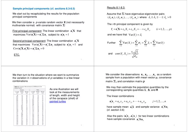
As one illustration we will look at the measurements

• f length, width and height
• f the carapace (shell) of

We then turn to the situation where we want to summarize the variation in n observations of p variables in a few linear combinations

3

• f the carapace (shell) of

painted turtles We may then estimate the population quantities by the corresponding sample quantities , S, and R The linear combinations We consider the observations x1, x2, .... ,xn as a random sample from a population with mean vector , covariance matrix Σ, and correlation matrix ρ

x

have sample mean and sample variance (cf. section 3.6)

4

1 11 1 12 2 1

1,2,....,

j j j p jp

a x a x a x j n ′ = + + + = a x ⋯

Also the pairs for two linear combinations have sample covariance

1 1

′ a Sa

1

′ a x

1 2

′ a Sa

1 2

( , )

j j

′ ′ a x a x

SLIDE 2

The sample principal components are the linear combinations which have maximum sample variance and sample covariance zero: First sample principal component: The linear combination that maximizes the sample variance of subject to

1 j

′ a x

1 1

1 ′ = a a

1 j

′ a x

5 5

sample variance of subject to

1 1

Second principal component: The linear combination that maximizes the sample variance of subject to and zero sample covariance for the pairs

2 2

1 ′ = a a

1 j

ETC.

2 j

′ a x

2 j

′ a x

1 2

( , )

j j

′ ′ a x a x

Assume that S have eigenvalue-eigenvector pairs where Result: The i-th sample principal component is given by

1 1 2 2

ˆ ˆ ˆ ˆ ˆ ˆ ( , ), ( , ), , ( , )

p p

λ λ λ e e e …

1 2

ˆ ˆ ˆ

p

λ λ λ ≥ ≥ ≥ > ⋯

1 1 2 2

ˆ ˆ ˆ ˆ ˆ ( 1,2, , )

i i i i ip p

y e x e x e x i p ′ = = + + + = e x ⋯ …

also and the sample covariance

ˆ ˆ sample variance( ) y λ =

6

also and the sample covariance

• f the pairs is zero

Further

1 1

ˆ total sample variance

p p ii i i i

s λ

= =

= =

∑ ∑

and

ˆ ˆ ˆ sample correlation( , )

ik i i k kk

e y x s λ = ˆ ˆ sample variance( )

i i

y λ = ˆ ˆ ( , ), ,

i k

y y i k ≠

The observations are often “centered” by subtracting

j

x x

This has no effect on S, and hence no effect on the eigenvalues/eigenvectors The “centered” principal components become

ˆ ˆ ( ) ( 1,2, , )

i i

y i p ′ = − = e x x …

7

ˆ ˆ ( ) ( 1,2, , )

i i

y i p ′ = − = e x x …

The values of the i-th “centered” principal component are

ˆ ˆ ( ) ( 1,2, , )

ji i j

y j n ′ = − = e x x …

Note that

1 1

1 1 ˆ ˆ ˆ ( )

n n ji ji j j j

y y n n

= =

′ = = − =

∑ ∑

e x x

Example 8.4 Measurements of length, width and height of the carapace (shell) of male painted turtles

8

SLIDE 3

Example 8.4 Socioeconomic variables in census tracts for the Madison, Wisconsin, area

9

Observations that are on different scales are often standardized:

1 1 2 2 11 22

, , , ( 1,2, , )

j j jp p j pp

x x x x x x j n s s s ′   − − −   = =     z … …

10

 

Note that the standardized observations are “centered” and that their covariance matrix is the correlation matrix R Assume that R have eigenvalue-eigenvector pairs where Result for standardized observations: The i-th sample principal component is given by

1 1 2 2

ˆ ˆ ˆ ˆ ˆ ˆ ( , ), ( , ), , ( , )

p p

λ λ λ e e e …

1 2

ˆ ˆ ˆ

p

λ λ λ ≥ ≥ ≥ > ⋯

1 1 2 2

ˆ ˆ ˆ ˆ ˆ ( 1,2, , )

i i i i ip p

y e z e z e z i p ′ = = + + + = e z ⋯ …

also and the sample covariance

ˆ ˆ sample variance( ) y λ =

11

also and the sample covariance

• f the pairs is zero

Further

1

ˆ total sample variance

p i i

p λ

=

= =∑

and

ˆ ˆ ˆ sample correlation( , )

i k ik i

y z e λ = ˆ ˆ sample variance( )

i i

y λ = ˆ ˆ ( , ), ,

i k

y y i k ≠

Example 8.5 Weekly rates of return for five stocks on New York Stock Exchange Jan 2004 through Dec 2005

12

SLIDE 4

Plots of principal components may help to detect suspect observations and provide check for multivariate normality The principal components are linear combinations of the original variables, so they should be (approximately) independent and normally distributed if the original observations are multivariate normal

13

This may be checked by making normal probability plots and scatter plots of the observed values of the principal components Then the sample principal components Assume now that the observations x1, x2, .... ,xn independent realizations from a multivariate normal distribution with mean vector , covariance matrix Σ

ˆ ˆ ( ) ( 1,2, , ; 1,2, , )

ji i j

y i p j n ′ = − = = e x x … …

are realizations of the population principal components

14

( ) ( 1,2, , )

i i

Y i p ′ = − = e X

• …

Also these population principal components are independent and normally distributed with means zero and variances given by the eigenvalues of the covariance matrix Σ

i

λ

What are the properties of the and the considered as estimators of the and the ?

ˆ '

i s

λ ˆ '

i s

e '

i s

λ '

i s

e

Assume now that our observations are independent realizations from a multivariate normal distribution one may prove the following results for large samples (i.e. large n) The sample eigenvalues are approximately independent and

2

ˆ ( ,2 / ) approximately N n λ λ λ ∼

15

2

ˆ ( ,2 / ) approximately

i i i

N n λ λ λ ∼ ˆ ( , / ) approximately

i p i i

N n e e E ∼

where

2 1 (

)

p k i i k k k k i k ì

λ λ λ λ

= ≠

′ = −

∑

E e e