The (Horse) Flys Eye A Search for Highly Energetic Radio Pulses - - PowerPoint PPT Presentation

The (Horse) Fly’s Eye

Geoff Bower, Jim Cordes, Griffin Foster, Joeri van Leeuwen, William Mallard, Peter McMahon, Andrew Siemion, Mark Wagner, Dan Werthimer

A Search for Highly Energetic Radio Pulses from Extragalactic Sources using the Allen Telescope Array

CASPER Workshop II 08.04.08 Griffin Foster, Andrew Siemion, Peter McMahon

Motivation

Parkes Multibeam Pointing During Lorimer Detection Frequency vs. Time Waterfall for Lorimer Detection

• Announced September 2007
• Single pulse at L-band
• 30 Jy, saturated digitizer in one beam
• Located 3° from the SMC
• DM = 375 pc/cm3 implies D ~ 1Gpc

Exciting Results From Lorimer et al.

• Lorimer, et. al., “A Bright Millisecond Radio Burst of Extragalatic Origin.” Science, 318, 2007.

The Fly’s Eye: The Search for HERPES

• Highly Energetic Radio Pulses for Extragalactic Sources
• Goal: Build a set of 44 independent spectrometers for the ATA and

use them to search for HERPES over a large portion of the sky.

• November 19, 2007 - Dan Werthimer and Geoff Bower have lunch to discuss a

suggestion made by Jim Cordes to perform a transient search using the ATA.

• November 20, 2007 - Dan Werthimer tasks a group of mostly undergraduate students

at the Center for Astronomy Signal Processing and Electronics Research (CASPER) to begin building a transient instrument.

• December 22, 2007 - Fly’s Eye Team installs Fly’s Eye at ATA.
• February, March 2008 - Conducted 500 hours of weekend observations.
• April - August... 2008 - Data analysis underway

Timeline

The Allen Telescope Array

• Located in Hat Creek, CA (~5 hours from Berkeley)
• 42 x 6 m dishes, 0.5-11 GHz usable band
• 4 independent tunable IFs
• First light was less then a year ago, October 2007 (Galaxy M31)
• Newly commissioned, so there is plenty of observing time available
• Each antenna has a wide beam, ~2° FWHM (at L band)
• With independent, tunable IFs commensal observing is very easy

Advantages Text

iBOB Spectrometer

Using standard CASPER libraries and the pocket correlator design the 4 input spectrometer used in Fly’s Eye was completed in 3 weeks.

The Instrument

44 independent spectrometers - constructed using a system of eleven iBOB/iADC quad spectrometers Built using open-source CASPER hardware and software libraries in about one month.

Sky Coverage: 22 - 42 beams 100-200 square degrees Spectrometer Specifications (each): 208 MHz bandwidth, at 1430 MHz 128 spectral channels 0.625 mS readout Distributions: Spatial, DM, Power, Pulse Width

Fly’s Eye Rack at ATA

PSR B0329+54 Detection

Instrument Diagnostics

PSR B0329+54 Detections in all 44 Beams (15 minutes folded) PSR B0329+54 (36 beams summed, 15 minutes folded)

PSR B0329+54 detected in 41/44 signal paths.

Control and Monitoring

After initial instrument setup at the ATA all observations were done remotely

Observation Diagnostics

32 64 96 128 10 20 30 40 50

ibob-g38

32 64 96 128 10 20 30 40 50

ibob-g39

32 64 96 128 10 20 30 40 50

ibob-g40

32 64 96 128 10 20 30 40 50

ibob-g41

32 64 96 128 10 20 30 40 50

ibob-g42

32 64 96 128 10 20 30 40 50

ibob-g43

32 64 96 128 10 20 30 40 50

ibob-g44

32 64 96 128 10 20 30 40 50

ibob-g45

32 64 96 128 10 20 30 40 50

ibob-g46

32 64 96 128 10 20 30 40 50

ibob-g47

32 64 96 128 10 20 30 40 50

ibob-g48

AA BB CC DD

• All observations were done via

scripts on a control machine and recorded to a data server (via gulp)

• For every hour of observations

58 minutes were used in the horseshoe pattern, 1 minutes was used for recording diagnostic data to assure data quality, note the 21 cm line.

• Packet loss statistics and

spectra from diagnostic runs were uploaded to a web server

Observations

Total observing time thus far is approximately 480 hours. Both North and South pointing

• bservations were performed,

primarily North due to kinder RFI environment. Total dataset is approximately 17 terabytes.

Fly’s Eye Beam Pointing Diagram

Drift scan Fly’s Eye observations were conducted in campaign mode on weekends between February and April 2008. Initial plan was for “fly’s eye” sky patch observing, eventually transformed to “horseshoe” constant declination strip.

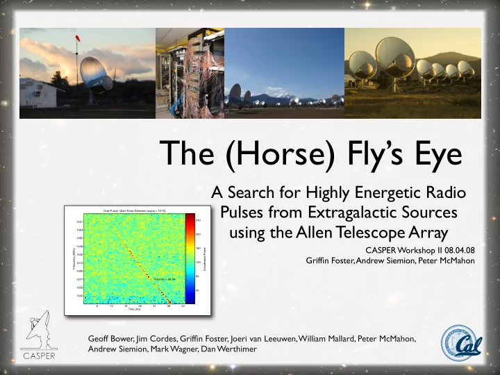
fitted dm = 56.78 Uncalibrated Power Crab Pulsar: Giant Pulse Detection (sigma = 15.75) Frequency (MHz) Time (ms) 6 13 19 25 31 38 44 1501 1483 1465 1448 1430 1412 1395 1377 1359 1342 40 80 120 160 200 240

Giant Pulses From PSR B0531+21

Instrument Diagnostics

Giant Pulses from PSR B0531+21 (35 beams) Giant Pulse from PSR B0531+21 (single beam)

The Crab pulsar has be well studied, and is know to produce giant

• pulses. The pulsar was observed for one hour, during which close

to a dozen detectable pulses were detected (in summed data), the brightest of which was distinguishable in approximately half of single dish observations.

Data Analysis

Raw gulp Datafile Error Analysis / Dropped Packet Correction IF Seperation (filterbank) IF 0 IF 1 IF 2 IF 43 IF SUM

....

De-dispersion DM 0 (dedisperse)

.... ....

Frequency Collapse (dedisperse) RFI Rejection

• freq. and time

domains Equalization / Normalization

.... ....

De-dispersion DM 1 (dedisperse) De-dispersion DM 2 (dedisperse)

....

De-dispersion DM 1000 (dedisperse) Compute RMS / Threshold (seek) Log Candidate Pulses Decimate (seek) Disk Storage (MySQL Database)

.... .... ....

• DM search range:

50-2000 pc/cm3 (with decimation, non-integer spacing)

• Computing grids used:

5 (Berkeley Wireless Research Center, UC Berkeley EECS, DOE NERSC)

• Total cores (peak):

~200 (Itanium64, Xeon, Sparc, Opteron)

• Total throughput (peak):

~200 Mbits/second

Fly’s Eye Data Analysis Pipeline

The RFI Challenge

Types of RFI:

• Wideband, short time period
• Narrowband, continuous(radio, airplanes, satellites)
• Narrowband, short time period(RADAR, more airplanes)
• Special cases(broken satellites?)

Solutions:

• Pre data analysis:
• normalization and equalization of spectra, remove

abnormal spectra(wideband RFI)

• time collapse and compute variance, similar to

kurtosis methods(narrowband, short time)

• Post data analysis:
• flag times with a wide range on DM events
• Special cases for low(<50 DM) and high(>1800 DM)

events

Current Challenges:

• RADAR
• Narrowband, short time period RFI
• Equalization/Normalization methods

The RFI Challenge: Military Radar

ARSR-4 Air Route Surveillance Radar

• Radar transmits on ~12s timescales
• With a low duty cycle the radar is hard to

remove using variance RFI removal

• In northern California there are 2 nearby sites

(Rainbow Ridge, Mill Valley)

• The stations operate out of phase with each
• ther and at different frequencies false high

DM detections

• Brute force solution: ignore these channels

Interesting RFI: Broken Satellites

After zooming in on the event we determined it was not terrestrial RFI or Aliens, but based on the angular speed of the object it is probably a low orbit satellite(transmitting around 1420 MHz!). From our first pass script we found ~80 interesting events, one event in particular looked like something we had never seen before, it was too narrow band to be wide band RFI and it was centered around 1420 MHz. (Aliens?!?!?!)

Then we zoomed in on the data...

Producing Results

MySQL Server

Post RFI Rejection Corrected Plots Raw Plots Decimated Waterfalls Web Interface Full Waterfalls Request Plots User Tag Events

• After data analysis the data is stored

to a MySQL server where our graphing pipeline retrieves data.

• Using Python we do RFI flagging and

generate a series of plots which can be viewed from a web interface

• The next step of the web interface

is to include user interaction to tag plots with i.e. interesting/bad rfi/ nothing...

• To view an interesting portion of the

data we retrieve the raw data from the tape backup, and generate a large waterfall plot of all the data for a time period (the large files sizes of

• ur data causes this step to take

~10 minutes to generate).

Example Preliminary Results

Example Time vs. Sigma Plot Example Time vs. DM Plot Result Browser

480 hours of

• bservations, 44

spectrometers, 10 minute sets, 9 plot types over a million plots!

New and Future Analysis

• We have the plot, now we need the eyes! Using our first pass

scripts we can find the interesting events in the best data but there is much more to be looked at.

• Reprocess! - Improve RFI rejection and implement new pulse

search algorithms (underway)

• Improve SNR in some of the data by summing polarizations
• Include a measurement of the kurtosis to remove intermittent

narrowband RFI

• Try different equalization techniques
• Improve speed of analysis

Assessment of Significance

Parameter Space for Radio Transient Detection

Region allowed by existing experiments Parameter space explored by Fly’s Eye I (Spring 2008) Parameter space potentially explored by a

• ne-year

commensal Fly’s Eye Experiment

Future Experiments: Localizing HERPES

Angular Localization of Transient Radio Bursts

• If we can find them, we should try and localize them.
• We can easily convert a 4 input iBOB Spectrometer to a

4 input Pocket Correlator

Fly’s Eye 44 input fast readout spectrometer becomes... Fly’s Eye 11 x 4 input fast readout correlator