The EM Algorithm The EM algorithm Mixture models Why EM works EM - PDF document

Preview The EM Algorithm • The EM algorithm • Mixture models • Why EM works • EM variants Learning with Missing Data The EM Algorithm • Goal: Learn parameters of Bayes net with known structure Initialize parameters ignoring missing information • For now: Maximum likelihood Repeat until convergence: • Suppose the values of some variables in some samples E step: Compute expected values of unobserved variables, are missing assuming current parameter values • If we knew all values, computing parameters would be M step: Compute new parameter values to maximize easy probability of data (observed & estimated) • If we knew the parameters, we could infer the missing values (Also: Initialize expected values ignoring missing info) • “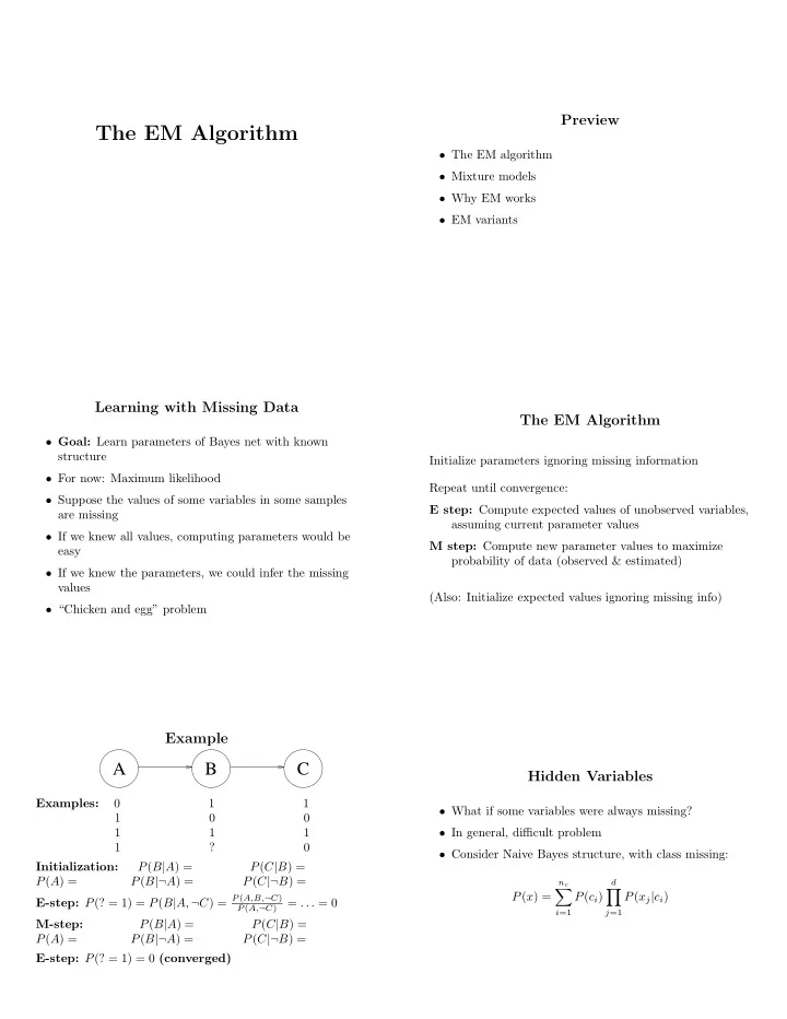Chicken and egg” problem Example A B C Hidden Variables Examples: 0 1 1 • What if some variables were always missing? 1 0 0 1 1 1 • In general, difficult problem 1 ? 0 • Consider Naive Bayes structure, with class missing: Initialization: P ( B | A ) = P ( C | B ) = P ( A ) = P ( B |¬ A ) = P ( C |¬ B ) = n c d � � P ( x ) = P ( c i ) P ( x j | c i ) E-step: P (? = 1) = P ( B | A, ¬ C ) = P ( A,B, ¬ C ) = . . . = 0 P ( A, ¬ C ) i =1 j =1 M-step: P ( B | A ) = P ( C | B ) = P ( A ) = P ( B |¬ A ) = P ( C |¬ B ) = E-step: P (? = 1) = 0 (converged)

Naive Bayes Model P ( Bag= 1) Clustering Bag C P ( F=cherry | B ) • Goal: Group similar objects Bag 1 • Example: Group Web pages with similar topics F 1 2 F 2 • Clustering can be hard or soft • What’s the objective function? X Flavor Wrapper Holes (a) (b) Mixtures of Gaussians Mixture Models n c � P ( x ) = P ( c i ) P ( x | c i ) i =1 p(x) Objective function: Log likelihood of data Naive Bayes: P ( x | c i ) = � n d j =1 P ( x j | c i ) AutoClass: Naive Bayes with various x j models x Mixture of Gaussians: P ( x | c i ) = Multivariate Gaussian � � 2 � 1 − 1 � x − µ i √ P ( x | µ i ) = 2 πσ 2 exp In general: P ( x | c i ) can be any distribution 2 σ EM for Mixtures of Gaussians Simplest case: Assume known priors and covariances Mixtures of Gaussians (cont.) Initialization: Choose means at random E step: For all samples x k : • K-means clustering ≺ EM for mixtures of Gaussians P ( µ i | x k ) = P ( µ i ) P ( x k | µ i ) P ( µ i ) P ( x k | µ i ) • Mixtures of Gaussians ≺ Bayes nets = P ( x k ) � i ′ P ( µ i ′ ) P ( x k | µ i ′ ) • Also good for estimating joint distribution of continuous variables M step: For all means µ i : � x k x P ( µ i | x k ) µ i = � x k P ( µ i | x k )

Why EM Works LL(Onew) EM Variants MAP: Compute MAP estimates instead of ML in M step LL(Onew) LLold GEM: Just increase likelihood in M step MCMC: Approximate E step LLold + Q(Onew) Simulated annealing: Avoid local maxima Early stopping: Faster, may reduce overfitting Oold Onew Structural EM: Missing data and unknown structure θ new = argmax E θ old [log P ( X )] θ Summary • The EM algorithm • Mixture models • Why EM works • EM variants