Expectation maximization don't have any labels. Can you still do - - PowerPoint PPT Presentation

SLIDE 1

Subhransu Maji

CMPSCI 689: Machine Learning

14 April 2015

Expectation maximization

Subhransu Maji (UMASS) CMPSCI 689 /19

Suppose you are building a naive Bayes spam classifier. After your are done your boss tells you that there is no money to label the data.!

• You have a probabilistic model that assumes labelled data, but you

don't have any labels. Can you still do something?

!

Amazingly you can!!

• Treat the labels as hidden variables and try to learn them

simultaneously along with the parameters of the model

!

Expectation Maximization (EM) !

• A broad family of algorithms for solving hidden variable problems
• In today’s lecture we will derive EM algorithms for clustering and

naive Bayes classification and learn why EM works

Motivation

2 Subhransu Maji (UMASS) CMPSCI 689 /19

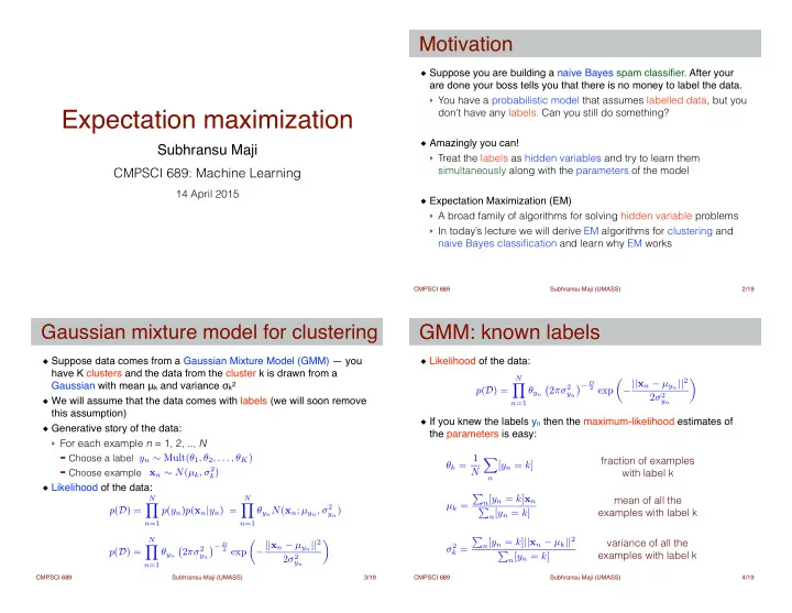
Suppose data comes from a Gaussian Mixture Model (GMM) — you have K clusters and the data from the cluster k is drawn from a Gaussian with mean μk and variance σk2! We will assume that the data comes with labels (we will soon remove this assumption)! Generative story of the data:!

• For each example n = 1, 2, .., N

➡ Choose a label ➡ Choose example

Likelihood of the data:

Gaussian mixture model for clustering

3

xn ∼ N(µk, σ2

k)

yn ∼ Mult(θ1, θ2, . . . , θK) p(D) =

N

Y

n=1

p(yn)p(xn|yn) =

N

Y

n=1

θynN(xn; µyn, σ2

yn)

p(D) =

N

Y

n=1

θyn

• 2πσ2

yn

− D

2 exp

✓ −||xn − µyn||2 2σ2

yn

◆

Subhransu Maji (UMASS) CMPSCI 689 /19

Likelihood of the data:!

! ! !

If you knew the labels yn then the maximum-likelihood estimates of the parameters is easy:

GMM: known labels

4

θk = 1 N X

n

[yn = k] µk = P

n[yn = k]xn

P

n[yn = k]

fraction of examples with label k mean of all the examples with label k variance of all the examples with label k p(D) =

N

Y

n=1

θyn

• 2πσ2

yn

− D

2 exp

✓ −||xn − µyn||2 2σ2

yn

◆ σ2

k =

P

n[yn = k]||xn − µk||2

P

n[yn = k]

SLIDE 2

Subhransu Maji (UMASS) CMPSCI 689 /19

Now suppose you didn’t have labels yn. Analogous to k-means, one solution is to iterate. Start by guessing the parameters and then repeat the two steps:!

• Estimate labels given the parameters
• Estimate parameters given the labels

!

In k-means we assigned each point to a single cluster, also called as hard assignment (point 10 goes to cluster 2)! In expectation maximization (EM) we will will use soft assignment (point 10 goes half to cluster 2 and half to cluster 5)!

!

Lets define a random variable zn = [z1, z2, …, zK] to denote the assignment vector for the nth point!

• Hard assignment: only one of zk is 1, the rest are 0
• Soft assignment: zk is positive and sum to 1

GMM: unknown labels

5 Subhransu Maji (UMASS) CMPSCI 689 /19

Formally zn,k is the probability that the nth point goes to cluster k!

! ! ! ! !

Given a set of parameters (θk,μk,σk2), zn,k is easy to compute! Given zn,k , we can update the parameters (θk,μk,σk2) as:

GMM: parameter estimation

6

zn,k = p(yn = k|xn) = P(yn = k, xn) P(xn) ∝ P(yn = k)P(xn|yn) = θkN(xn; µk, σ2

k)

θk = 1 N X

n

zn,k µk = P

n zn,kxn

P

n zn,k

σ2

k =

P

n zn,k||xn − µk||2

P

n zn,k

fraction of examples with label k mean of all the fractional examples with label k variance of all the fractional examples with label k

Subhransu Maji (UMASS) CMPSCI 689 /19

We have replaced the indicator variable [yn = k] with p(yn=k) which is the expectation of [yn=k]. This is our guess of the labels.! Just like k-means the EM is susceptible to local minima.! Clustering example:

GMM: example

7

http://nbviewer.ipython.org/github/NICTA/MLSS/tree/master/clustering/

k-means GMM

Subhransu Maji (UMASS) CMPSCI 689 /19

We have data with observations xn and hidden variables yn, and would like to estimate parameters θ! The likelihood of the data and hidden variables:!

! !

Only xn are known so we can compute the data likelihood by marginalizing out the yn:!

! ! !

Parameter estimation by maximizing log-likelihood:

The EM framework

8

hard to maximize since the sum is inside the log

p(D) = Y

n

p(xn, yn|θ) p(X|θ) = Y

n

X

yn

p(xn, yn|θ) θML ← arg max

θ

X

n

log X

yn

p(xn, yn|θ) !

SLIDE 3

Subhransu Maji (UMASS) CMPSCI 689 /19

Given a concave function f and a set of weights λi ≥ 0 and ∑ᵢ λᵢ = 1! Jensen’s inequality states that f(∑ᵢ λᵢ xᵢ) ≥ ∑ᵢ λᵢ f(xᵢ)! This is a direct consequence of concavity!

• f(ax + by) ≥ a f(x) + b f(y) when a ≥ 0, b ≥ 0, a + b = 1

Jensen’s inequality

9

f(x) f(y) a f(x) + b f(y) f(ax+by)

Subhransu Maji (UMASS) CMPSCI 689 /19

Construct a lower bound the log-likelihood using Jensen’s inequality!

! ! ! ! ! ! ! ! ! !

Maximize the lower bound:

The EM framework

10

θ ← arg max

θ

X

n

X

yn

q(yn) log p(xn, yn|θ) independent of θ L(X|θ) = X

n

log X

yn

p(xn, yn|θ) ! = X

n

log X

yn

q(yn)p(xn, yn|θ) q(yn) ! ≥ X

n

X

yn

q(yn) log ✓p(xn, yn|θ) q(yn) ◆ = X

n

X

yn

[q(yn) log p(xn, yn|θ) − q(yn) log q(yn)] , ˆ L(X|θ)

x

λ

Jensen’s inequality

f

Subhransu Maji (UMASS) CMPSCI 689 /19

Maximizing the lower bound increases the value of the original function if the lower bound touches the function at the current value

Lower bound illustrated

11

L(X|θ) θt θt+1 ˆ L(X|θt) ˆ L(X|θt+1)

Subhransu Maji (UMASS) CMPSCI 689 /19

Any choice of the probability distribution q(yn) is valid as long as the lower bound touches the function at the current estimate of θ"

!

We can the pick the optimal q(yn) by maximizing the lower bound!

! !

This gives us!

• Proof: use Lagrangian multipliers with “sum to one” constraint

!

This is the distributions of the hidden variables conditioned on the data and the current estimate of the parameters!

• This is exactly what we computed in the GMM example

An optimal lower bound

12

L(X|θt) = ˆ L(X|θt) q(yn) ← p(yn|xn, θt) arg max

q

X

yn

[q(yn) log p(xn, yn|θ) − q(yn) log q(yn)]

SLIDE 4

Subhransu Maji (UMASS) CMPSCI 689 /19

We have data with observations xn and hidden variables yn, and would like to estimate parameters θ of the distribution p(x | θ)! EM algorithm!

• Initialize the parameters θ randomly
• Iterate between the following two steps:

➡ E step: Compute probability distribution over the hidden variables

!

➡ M step: Maximize the lower bound

! ! !

EM algorithm is a great candidate when M-step can done easily but p(x | θ) cannot be easily optimized over θ!

• For e.g. for GMMs it was easy to compute means and variances

given the memberships

The EM algorithm

13

q(yn) ← p(yn|xn, θ) θ ← arg max

θ

X

n

X

yn

q(yn) log p(xn, yn|θ)

Subhransu Maji (UMASS) CMPSCI 689 /19

Consider the binary prediction problem! Let the data be distributed according to a probability distribution:!

! !

We can simplify this using the chain rule of probability:!

! ! ! !

Naive Bayes assumption:!

! ! !

E.g., The words “free” and “money” are independent given spam

Naive Bayes: revisited

14

pθ(y, x) = pθ(y, x1, x2, . . . , xD)

pθ(y, x) = pθ(y)pθ(x1|y)pθ(x2|x1, y) . . . pθ(xD|x1, x2, . . . , xD−1, y) = pθ(y)

D

Y

d=1

pθ(xd|x1, x2, . . . , xd−1, y)

pθ(xd|xd0, y) = pθ(xd|y), 8d0 6= d

Subhransu Maji (UMASS) CMPSCI 689 /19

Case: binary labels and binary features!

! ! ! !

Probability of the data:

Naive Bayes: a simple case

15

pθ(y) = Bernoulli(θ0) pθ(xd|y = 1) = Bernoulli(θ+

d )

pθ(xd|y = −1) = Bernoulli(θ−

d )

1+2D parameters

}

// label +1 // label -1

pθ(y, x) = pθ(y)

D

Y

d=1

pθ(xd|y) = θ[y=+1] (1 − θ0)[y=−1] ... ×

D

Y

d=1

θ+[xd=1,y=+1]

d

(1 − θ+

d )[xd=0,y=+1]

... ×

D

Y

d=1

θ−[xd=1,y=−1]

d

(1 − θ−

d )[xd=0,y=−1]

Subhransu Maji (UMASS) CMPSCI 689 /19

Given data we can estimate the parameters by maximizing data likelihood! The maximum likelihood estimates are:

Naive Bayes: parameter estimation

16

ˆ θ0 = P

n[yn = +1]

N

// fraction of the data with label as +1 // fraction of the instances with 1 among +1

ˆ θ−

d =

P

n[xd,n = 1, yn = −1]

P

n[yn = −1]

ˆ θ+

d =

P

n[xd,n = 1, yn = +1]

P

n[yn = +1] // fraction of the instances with 1 among -1

SLIDE 5

Subhransu Maji (UMASS) CMPSCI 689 /19

Now suppose you don’t have labels yn! Initialize the parameters θ randomly! E step: compute the distribution over the hidden variables q(yn)!

! !

M step: estimate θ given the guesses

Naive Bayes: EM

17

q(yn = 1) = p(yn = +1|xn, θ) ∝ θ+

D

Y

d=1

θ+[xd,n=1]

d

(1 − θ+

d )[xd,n=0]

θ0 = P

n q(yn = 1)

N θ+

d =

P

n[xd,n = 1]q(yn = 1)

P

n q(yn = 1)

θ−

d =

P

n[xd,n = 1]q(yn = −1)

P

n q(yn = −1)

// fraction of the data with label as +1 // fraction of the instances with 1 among +1 // fraction of the instances with 1 among -1

Subhransu Maji (UMASS) CMPSCI 689 /19

Expectation maximization!

• A general technique to estimate parameters of probabilistic models

when some observations are hidden

• EM iterates between estimating the hidden variables and
• ptimizing parameters given the hidden variables
• EM can be seen as a maximization of the lower bound of the data

log-likelihood — we used Jensen’s inequality to switch the log-sum to sum-log EM can be used for learning:!

• mixtures of distributions for clustering, e.g. GMM
• parameters for hidden Markov models (next lecture)
• topic models in NLP
• probabilistic PCA
• ….

Summary

18 Subhransu Maji (UMASS) CMPSCI 689 /19

Some of the slides are based on CIML book by Hal Daume III! The figure for the EM lower bound is based on https:// cxwangyi.wordpress.com/2008/11/! Clustering k-means vs GMM is from http://nbviewer.ipython.org/ github/NICTA/MLSS/tree/master/clustering/

Slides credit

19