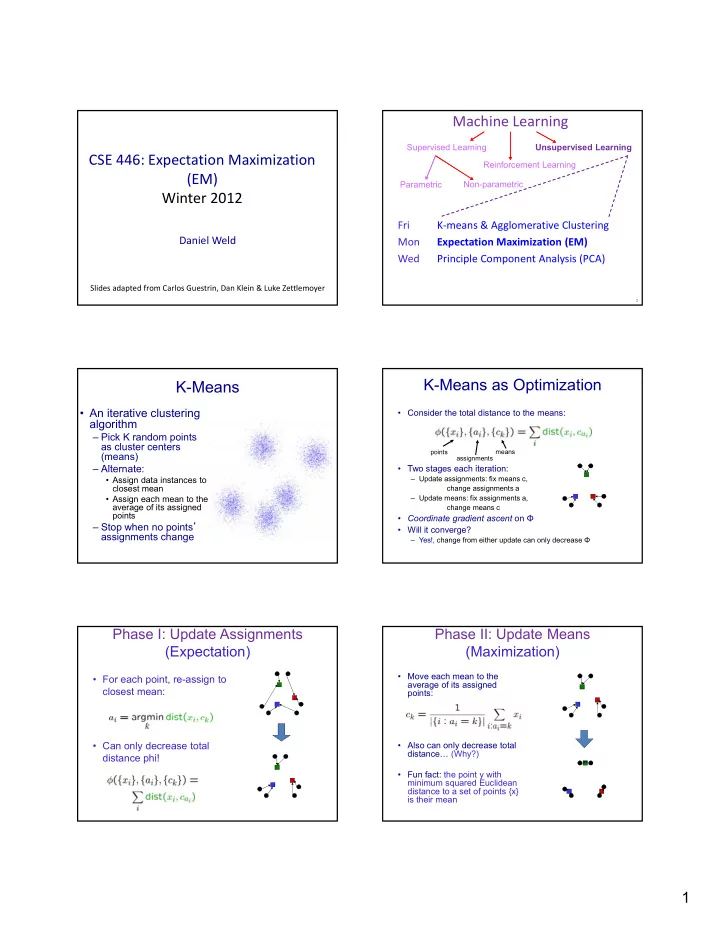
Machine Learning Supervised Learning Unsupervised Learning CSE 446: - PDF document

Machine Learning Supervised Learning Unsupervised Learning CSE 446: Expectation Maximization Reinforcement Learning (EM) Parametric Non-parametric Winter 2012 Fri K ‐ means & Agglomerative Clustering Daniel Weld Mon Expectation Maximization (EM) Wed Principle Component Analysis (PCA) Slides adapted from Carlos Guestrin, Dan Klein & Luke Zettlemoyer 2 K-Means as Optimization K-Means • An iterative clustering • Consider the total distance to the means: algorithm – Pick K random points as cluster centers means points (means) assignments – Alternate: Alt t • Two stages each iteration: T t h it ti • Assign data instances to – Update assignments: fix means c, closest mean change assignments a • Assign each mean to the – Update means: fix assignments a, average of its assigned change means c points • Coordinate gradient ascent on Φ – Stop when no points ’ • Will it converge? assignments change – Yes!, change from either update can only decrease Φ Phase I: Update Assignments Phase II: Update Means (Expectation) (Maximization) • Move each mean to the • For each point, re-assign to average of its assigned closest mean: points: • Can only decrease total • Also can only decrease total distance… (Why?) distance phi! • Fun fact: the point y with minimum squared Euclidean distance to a set of points {x} is their mean 1

K-Means Getting Stuck Preview: EM another iterative clustering algorithm A local optimum: • Pick K random cluster models • Alternate: – Assign data instances Assign data instances proportionately to different models – Revise each cluster model based on its (proportionately) assigned points • Stop when no changes Why doesn ’ t this work out like the earlier example, with the purple taking over half the blue? Preference for Equally Sized Clusters The Evils of “ Hard Assignments ”? • Clusters may overlap • Some clusters may be “wider” than others • Distances can be deceiving! 9 Probabilistic Clustering The General GMM assumption • P(Y): There are k components • Try a probabilistic model! • P(X|Y): Each component generates data from a multivariate Y X 1 X 2 Gaussian with mean μ i and covariance matrix  i • allows overlaps, clusters of different size, etc. ?? 0.1 2.1 Each data point is sampled from a generative process : • Can tell a generative story for ?? 0.5 ‐ 1.1 1. Choose component i with probability P(y=i) data Generate datapoint ~ N( m i ,  i ) 2. ?? 0.0 3.0 – P(X|Y) P(Y) is common   ?? ‐ 0.1 ‐ 2.0 • Challenge: we need to estimate   ?? 0.2 1.5 model parameters without labeled Ys   … … … 2

What Model Should We Use? Could we make fewer assumptions? • Depends on X! Y X 1 X 2 • Here, maybe Gaussian Naïve Bayes? ?? 0.1 2.1 • What if the X i co ‐ vary? – Multinomial over clusters Y • What if there are multiple peaks? ?? 0.5 ‐ 1.1 – Gaussian over each X i given Y i g • Gaussian Mixture Models! ?? 0.0 3.0 – P(Y) still multinomial ?? ‐ 0.1 ‐ 2.0 – P( X |Y) is a multivariate Gaussian dist’n ?? 0.2 1.5  T  i  (2  ) m /2 ||  i || 1/2 exp  1 1     P ( X  x j | Y  i )  2 x j   i  1 x j   i … … …     Review: Gaussians The General GMM assumption 1.What’s a Multivariate Gaussian? 2.What’s a Mixture Model ?       Learning Gaussian Parameters Multivariate Gaussians (given fully ‐ observable data) Eigenvalue, λ Covariance matrix, Σ , = degree to which x i vary together g  T  i  (2  ) m /2 ||  i || 1/2 exp  1 1     P ( X  x j | Y  i )  2 x j   i  1 x j   i P(X= x j )=     18 3

Multivariate Gaussians Multivariate Gaussians Σ  identity matrix Σ = diagonal matrix X i are independent ala Gaussian NB 19 20 Multivariate Gaussians The General GMM assumption 1.What’s a Multivariate Gaussian? 2.What’s a Mixture Model ?     Σ = arbitrary (semidefinite) matrix specifies rotation (change of basis)   eigenvalues specify relative elongation 21 Mixtures of Gaussians (1) Mixtures of Gaussians (1) Old Faithful Data Set Old Faithful Data Set ruption Time to Er Duration of Last Eruption Single Gaussian Mixture of two Gaussians 4

Mixtures of Gaussians (2) Mixtures of Gaussians (3) Combine simple models into a complex model: Component Mixing coefficient K=3 Eliminating Hard Assignments to Clusters Eliminating Hard Assignments to Clusters Model data as mixture of multivariate Gaussians Model data as mixture of multivariate Gaussians Eliminating Hard Assignments to Clusters Detour/Review: Supervised MLE for GMM Model data as mixture of multivariate Gaussians • How do we estimate parameters for Gaussian Mixtures with fully supervised data? • Have to define objective and solve optimization problem.  T  i  1 || 1/2 exp  1 x j   i         P ( y  i , x j )   i  1 x j   i  i  P ( y  i ) ( y , j ) p  ( y )   (2  ) m /2 ||  i || 1/2 ) m /2 ||   j i j   ( 2 • For example, MLE estimate has closed form solution: n  ML  1  n  ML  1    x j  ML   x n T x j  ML n n j  1 j  1 π i = probability point was generated from i th Gaussian 5

That was easy! Compare But what if unobserved data ? • Univariate Gaussian • MLE: – argmax θ  j P(y j ,x j ) – θ : all model parameters • eg, class probs, means, and variance for naïve Bayes • Mixture of Multi variate Gaussians • But we don’t know y j ’s!!! • Maximize marginal likelihood :  ML  1 n n   ML  1    x j  ML   k P(y j =i,x j ) T – argmax θ  j P(x j ) = argmax  j  i=1 x n x j  ML n n j  1 j  1 Simple example: learn means only! How do we optimize? Closed Form? Consider: P • Maximize marginal likelihood : • 1D data – argmax θ  j P(x j ) = argmax  j  i=1 k P(y j =i,x j ) • Mixture of k=2 Gaussians • Almost always a hard problem! • Variances fixed to σ =1 – Usually no closed form solution Usually no closed form solution • Dist n over classes is uniform • Dist’n over classes is uniform – Even when P(X,Y) is convex, P(X) generally isn’t… • Just estimate μ 1 and μ 2 -3 -2 -1 0 1 2 3 – For all but the simplest P(X), we will have to do gradient ascent, in a big messy space with lots of local optimum…   m k m k exp  1     P ( x , y  i )  2  2 x   i 2  P ( y  i )    j  1 i  1 j  1 i  1 μ 2 Marginal Likelihood Learning general mixtures of Gaussian for Mixture of two Gaussians  T  i  1 1/ 2 exp  1      1 x j   i P ( y  i | x j )  2 x j   i P ( y  i )   (2  ) m / 2 ||  i ||   • Marginal likelihood: Graph of μ 1 m m k    P ( x j )  P ( x j , y  i ) log P( x 1 , x 2 .. x n | μ 1 , μ 2 ) g ( 1 , n | μ 1 , μ 2 ) 2 j  1 j  1 i  1 against μ 1 and μ 2 m k  T  i  1 1/ 2 exp  1        2 x j   i  1 x j   i P ( y  i )   (2  ) m / 2 ||  i ||   j  1 i  1 • Need to differentiate and solve for μ i , Σ i , and P(Y=i) for i=1..k Max likelihood = ( μ 1 =-2.13, μ 2 =1.668) • There will be no closed for solution, gradient is complex, lots of Local minimum, but very close to global at ( μ 1 =2.085, μ 2 =-1.257)* local optimum • Wouldn’t it be nice if there was a better way!?! * corresponds to switching y 1 with y 2 . 6