SLIDE 1
The Determinant of a Square Matrix [AR 2.1–2.3]
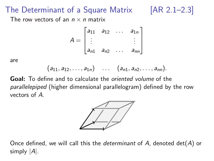
The row vectors of an n × n matrix A = a11 a12 . . . a1n . . . . . . an1 an2 . . . ann are (a11, a12, . . . , a1n) . . . (an1, an2, . . . , ann). Goal: To define and to calculate the oriented volume of the parallelepiped (higher dimensional parallelogram) defined by the row vectors of A. Once defined, we will call this the determinant of A, denoted det(A) or simply |A|.
SLIDE 2 Some 2-dimensional examples
The parallelograms of the row vectors of (3,0) (2,2) A = 3 2 2
B = 3 2
(0,2) have the same surface area, namely 3 · 2 = 6.
SLIDE 3 Examples for orientation
(1,0) (0,1) 1 1
- counter clock-wise orienta-
tion, the oriented surface area equals 1 (1,0) (0,1)
1
- clock-wise orientation, the
- riented surface area equals
- 1
versus In 3 dimensions: 1 1 1 gives a right- handed system with oriented vol- ume 1 1 1 1 gives a left- handed system with oriented vol- ume -1
SLIDE 4 Postulate
We want the assignment A − → det(A) to have the following properties:
- 1. If B is obtained from A by swapping two rows of A, then
det(B) = − det(A)
- 2. If B is obtained from A by multiplying a row of A by the scalar α,
then det(B) = α det(A)
- 3. If B is obtained from A by replacing a row of A by itself plus a
multiple of another row, then det(B) = det(A)
- 4. The determinant of any identity matrix is equal to 1.
We yet need to convince ourselves that such a function A → det(A) actually exists and that it is completely characterized by these
- properties. Then we will be allowed to use this slide as definition of
det(A). Computer lab 3 will cover determinants as volume and the effect of row
SLIDE 5
How to calculate determinants
Using the properties of the previous slide, det(A) is calculated as follows: If A is a triangular matrix, then det(A) is the product of the entries on the main diagonal of A. Examples 2 −1 9 3 2 2 2 1 3 2 −3 2 2 3 2 For a general matrix, do Gauss elimination to bring A into row echelon form, keeping track of what each step does to the determinant (it is best to avoid the 2nd elementary row operation). This is by far the sturdiest method for calculating determinants. The other methods are almost guaranteed to produce sign mistakes!
SLIDE 6 Examples Calculate
2 1 −1 −1 1 1 3
−4 1 3 −6 3 2 1 4
Calculate
−2 1 3 1 2 1 1 2 −2 1 2
−10 92 −117 3 28 −31 −1 27 2
- The determinant of a 2 × 2 matrix is ad − bc.
Proof: if a = 0
b c d
b d − cb
a
ad − bc and if a = 0
c d
−
d b
−bc.
SLIDE 7 Leibniz formula
A powerful theorem by Leibniz, which we will not pretend to prove, says that det(A) =
n
sgn(σ) ai,σ(i) satisfies the properties we postulated above. You will not be asked to calculate anything using Leibniz’ formula. To explain the symbols: the sum ranges over all shuffles (permutations) of {1, . . . , n} and sgn(σ) = ±1 depends on the number of flips in the shuffle σ. (Even that sgn(σ) is well-defined is a non-trivial fact.) We have already seen how to calculate the determinant, but it was not at all clear why two different ways to do Gauss elimination would yield the same result. This is one great thing about Leibniz’ definition: it is given directly in terms of A.
SLIDE 8 Other important properties of the determinant
= det(A)
- 6. det(AB) = det(A) det(B)
- 7. if A is an n × n matrix then det(αA) = αn det(A)
- 8. If A has a row (or column) of zeros, then det(A) = 0
- 9. If A has a row (or column) which is a scalar multiple of another
row (or column) then det(A) = 0
- 10. A is singular if and only if det(A) = 0
- 11. A is invertible if and only if det(A) = 0, and in this case
det
=
1 det(A)
C ∗ D
- with C, D square, then det(A) = det(C) det(D)
SLIDE 9 Additivity in the rows (Property 3’)
Determinants are not well behaved with respect to matrix addition. Example A = 1 1
2
1 1 2
Instead, we have: If the first row of C equals the sum of the first rows
- f A and B and all the other entries are identical in A, B and C then
det(C) = det(A) + det(B), and similarly for the ith row (or column). Example A = a b c d
a′ b′ c d
a + a′ b + b′ c d
SLIDE 10
Multilinearity
The property of the last slide looks similar to Property 2 (scaling a (single) row with a scalar α multiplies the determinant by the same scalar), and together these two properties are known as the multilinearity property of the determinant. Properties 1,2,3’ and 4 are often used to characterize the determinant. This approach is equivalent to our characterization by Properties 1-4. Idea of proof:
SLIDE 11 Laplace formula for det(A), a.k.a. cofactor expansion
The (i, j)-cofactor Cij of an n × n matrix A is the number Cij = (−1)i+j det (A(i, j)) where A(i, j) is the matrix obtained from A by deleting the ith row and jth column. To compute the determinant of A, choose any row (or column) of A, multiply each entry in that row (or column) by its cofactor and add the
- results. So, we obtain the cofactor expansion along the ith row:
det(A) = ai1Ci1 + ai2Ci2 + · · · + ainCin and the cofactor expansion along the jth column: det(A) = a1jC1j + a2jC2j + · · · + anjCnj
SLIDE 12 Examples If A = 1 2 1 −1 −1 1 1 3 , then A(2, 3) = 1 2 1
Calculate det 1 2 1 −1 −1 1 1 3 Calculate
−2 1 3 1 2 1 1 2 −2 1 2
- Cofactor expansion should be in your toolkit. Usually, Gauss
elimination works better, but if you can spot a column (or row) with many zeroes, go for cofactor expansion along it!
SLIDE 13
How do you remember the sign of the cofactor? The (1, 1)-cofactor always has sign +. Starting from there, imagine walking to the square you want using either horizontal or vertical steps. The appropriate sign will change at each step. We can visualize this arrangement with the following matrix: + − + − . . . − + − + . . . + − + − . . . − + − + . . . . . . . . . . . . . . . ... So, for example, C13 is assigned + but C32 is assigned −