Teaser: natural waters using wind-based wave generation Rendering - - PowerPoint PPT Presentation

Rendering Transparent and Turbid Fluids

PhD Course on the Deformable Simplicial Complex Method

Jeppe Revall Frisvad August 2010

To learn more about rendering, see http://www.imm.dtu.dk/courses/02576/

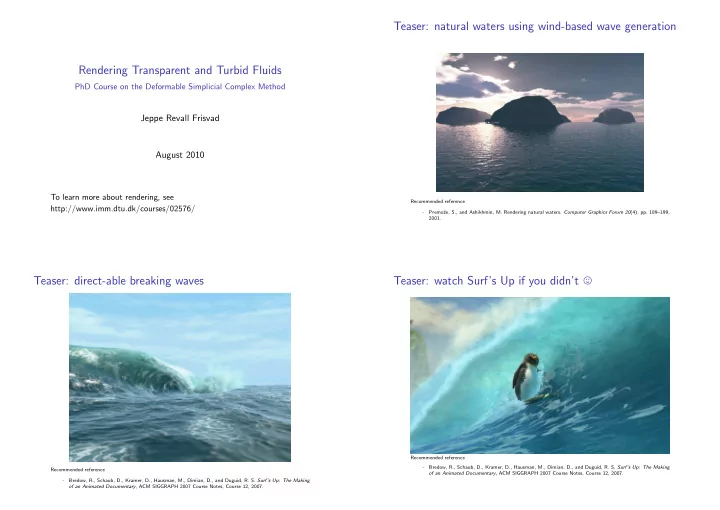
Teaser: natural waters using wind-based wave generation

Recommended reference

• Premoˇ

ze, S., and Ashikhmin, M. Rendering natural waters. Computer Graphics Forum 20(4), pp. 189–199, 2001.

Teaser: direct-able breaking waves

Recommended reference

• Bredow, R., Schaub, D., Kramer, D., Hausman, M., Dimian, D., and Duguid, R. S. Surf’s Up: The Making
• f an Animated Documentary, ACM SIGGRAPH 2007 Course Notes, Course 12, 2007.

Teaser: watch Surf’s Up if you didn’t

Recommended reference

• Bredow, R., Schaub, D., Kramer, D., Hausman, M., Dimian, D., and Duguid, R. S. Surf’s Up: The Making
• f an Animated Documentary, ACM SIGGRAPH 2007 Course Notes, Course 12, 2007.

Models needed for physically based rendering

◮ Think of the experiment: “taking a picture”. ◮ What do we need to model it?

◮ Camera ◮ Scene geometry ◮ Light sources ◮ Light propagation ◮ Materials

◮ Mathematical models for these physical phenomena are

required as a minimum in order to render an image.

◮ We can use very simple models, but, if we desire a high level

• f realism, more complicated models are required.

◮ To get started, we will go through the simpler models

(in opposite order).

Materials (scattering and absorption of light)

◮ Optical properties (index of refraction, n(λ) = n′(λ) + i n′′(λ)). ◮ Reflectance distribution functions, f (xi, xo,

ωi, ωo).

xi xo n1 n2 n1 n2

Light propagation

◮ Visible light is electromagnetic waves of wavelengths (λ) from

380 nm to 780 nm.

◮ Electromagnetic waves in transparent media propagate as rays

• f light for λ → 0.

◮ Rays of light follow the path of least time (Fermat). ◮ How does light propagate in air? In straight lines (almost). ◮ The parametrisation of a straight line in 3D is therefore a

good, simple model for light propagation.

Light sources

◮ A light source is described by a spectrum of light Le,λ(x,

ωo) which is emitted from each point on the emissive object.

◮ A simple model is a light source that from each point emits

the same amount of light in all directions and at all wavelengths, Le,λ = const.

◮ The spectrum of heat-based light sources can be estimated

using Planck’s law of radiation. Examples:

◮ The surface geometry of light sources is modelled in the same

way as other geometry in the scene.

Scene geometry

◮ Surface geometry is often modelled by a collection of triangles

some of which share edges (a triangle mesh).

◮ Triangles provide a discrete representation of an arbitrary

• surface. A quick example:

◮ Triangles are useful as they are defined by only three vertices.

And ray-triangle intersection is simple.

Examples of fluid geometry

Reference for the two renderings in the second row

• Bredow, R., Schaub, D., Kramer, D., Hausman, M., Dimian, D., and Duguid, R. S. Surf’s Up: The Making
• f an Animated Documentary, ACM SIGGRAPH 2007 Course Notes, Course 12, 2007.

Camera

◮ A camera consists of a light sensitive area, a processing unit,

and a storage for saving the captured images.

◮ The simplest model of a camera is a rectangle, which models

the light sensitive area (the chip/film), placed in front of an eye point where light is gathered.

◮ We can use this model in two different ways:

◮ Follow rays from the eye point through the rectangle and

• nwards (ray casting).

◮ Project the geometry on the image plane and find the

geometry that ends up in the rectangle (rasterization).

Ray casting

◮ Camera description:

Extrinsic parameters Intrinsic parameters e Eye point φ Vertical field of view p View point d Camera constant

• u

Up direction W , H Camera resolution

◮ Sketch of ray generation:

e p u v

image plane film ray pixel (i, j)

d h φ e

film

◮ For each ray, find the closest point where it intersects a triangle.

What is a ray?

◮ Parametrisation of a line: x(t) = e + t

r.

◮ Camera provides origin (e) and direction (

r) of “eye rays”.

◮ The user sets origin and direction when tracing rays recursively. ◮ But we need more properties:

◮ Maximum distance (max t) for visibility detection. ◮ Information about what was hit and where (hit normal,

position, distance, material, etc.).

◮ A counter to tell us the trace depth: how many reflections or

refractions the ray suffered from (no. of recursions).

Ray tracing

◮ What do you need in a ray tracer?

◮ Camera (ray generation and lens effects) ◮ Ray-object intersection (and accelleration) ◮ Light distribution (different source types) ◮ Visibility testing (for shadows) ◮ Surface scattering (reflection models) ◮ Recursive ray tracing (rays spawn new rays)

◮ How to use a ray tracer? Trace radiant energy. ◮ The energy travelling along a ray of direction

r = − ω is measured in radiance (flux per projected area per solid angle).

◮ The outgoing radiance Lo at a surface point x is the sum of

emitted radiance Le and reflected radiance Lr: Lo(x, ω) = Le(x, ω) + Lr(x, ω) .

◮ Reflected radiance is computed using the BRDF (fr) and an

estimate of incident radiance Li at the surface point.

The rendering equation

◮ Surface scattering is defined in terms of

◮ Radiance:

L = d2Φ cos θ dA dω .

◮ Irradiance:

E = dΦ dA , dE = L cos θ dω .

◮ BRDF:

fr(x, ω′, ω) = dLr(x, ω) dE(x, ω′) .

◮ The rendering equation then emerges from Lo = Le + Lr:

Lo(x, ω) = Le(x, ω) +

• 2π

fr(x, ω′, ω) Li(x, ω) cos θ′ dω′ .

◮ This is an integral equation. ◮ Integral equations are recursive in nature.

A Monte Carlo estimator for the rendering equation

◮ The rendering equation:

Lo(x, ω) = Le(x, ω) +

• 2π

fr(x, ω′, ω)Li(x, ω′) cos θ dω′ .

◮ The Monte Carlo estimator:

LN(x, ω) = Le(x, ω) + 1 N

N

• i=1

fr(x, ω′

i,

ω)Li(x, ω′

i) cos θ

pdf( ω′

i)

.

◮ The Lambertian (perfectly diffuse) BRDF:

fr(x, ω′, ω) = ρd/π .

◮ A good choice of pdf would be:

pdf( ω′

i) = cos θ/π .

Cosine-weighted hemisphere sampling

◮ Sampling directions according to the distribution:

pdf( ω′

i) = cos θ/π . ◮ In spherical coordinates: pdf(θ, φ) = cos θ sin θ/π . ◮ With two uniform random variables ξ1, ξ2 ∈ [0, 1], this pdf is

sampled by (θ, φ) = (cos−1 ξ1, 2πξ2) .

◮ In a local coordinate system, where the z-axis is the zenith

direction, the corresponding direction vector is (x, y, z) = (sin θ cos φ, sin θ sin φ, cos θ) .

◮ If we find an orthonormal basis {

b1, b2, n} which includes the surface normal n, we can rotate to world coordinates by a change of basis

• ω′

i = x

b1 + y b2 + z n .

Ambient occlusion

◮ Using the Lambertian BRDF for materials, fr = ρd/π; the

cosine weighted hemisphere for sampling, pdf( ω′

i) = cos θ/π;

and a visibility term V for incident illumination, the Monte Carlo estimator for ambient occlusion is simply: LN(x, ω) = 1 N

N

• i=1

fr(x, ω′

i,

ω)Li(x, ω′

i) cos θ

pdf( ω′

i)

= ρd(x) 1 N

N

• i=1

V ( ω′

i) .

Sampling a triangle mesh

◮ Uniformly sample a triangle (pdf = 1/n, where n is the

number of triangle faces in the mesh).

◮ Uniformly sample a position on the triangle (pdf = 1/A∆,

where A∆ is the triangle area):

• 1. Sample barycentric coordinates (u, v, w = 1 − u − v):

u = 1 −

• ξ1

v = (1 − ξ2)

• ξ1

w = ξ2

• ξ1
• 2. Use the barycentric coordinates for trilinear interpolation of

triangle vertices to obtain a point on the triangle.

• 3. Use the barycentric coordinates for trilinear interpolation of

triangle vertex normals to obtain the normal at the sampled surface point.

Soft shadows

◮ From solid angle to area: dω′ = cos θlight r2

dA.

◮ Using the Lambertian BRDF, fr = ρd/π, and triangle mesh

sampling of a point xi on the light, pdf = 1/(nA∆,i), the Monte Carlo estimator for area lights is: LN(x, ω) = ρd(x) π 1 N

N

• i=1

Le(xi → x)V (xi ↔ x)cos θ cos θlight x − xi2 nA∆,i .

The laws of reflection and refraction

n θ −n

r i

θr θt ni nt

t

ω’ ω ω

◮ The law of reflection (θr = θi)

• ωr = 2(

ω′ · n) n − ω′ .

◮ The law of refraction (ni sin θi = nt sin θt)

• ωt = ni

nt (( ω′ · n) − ω′) − n

• 1 −

ni nt 2 (1 − ( ω′ · n)2) .

Rendering transparent fluids

◮ Choose a maximum recursion depth. ◮ When the fluid is intersected:

◮ Trace a ray in the direction of the reflected ray. ◮ Trace a ray in the direction of the transmitted/refracted ray.

◮ But how much radiance is reflected and how much is

refracted?

Multiscale light modelling

◮ Light at different scales:

◮ Quantum electrodynamics (photons) ◮ Electromagnetic radiation (waves) ◮ Geometrical optics (rays) ◮ Radiative transfer (ray bundles)

◮ Why do we need to know? To understand:

◮ how light interacts with materials; ◮ where the material properties come from; ◮ when rays don’t work.

◮ Geometrical optics include:

◮ the law of reflection (Euclid ∼300 B.C. and before); ◮ the law of refraction (Ibn Sahl ∼984, Snel van Royen 1621).

◮ Electromagnetic radiation (Maxwell 1873) includes:

◮ the index of refraction; ◮ the amount of reflection and transmission at a specular surface

(Fresnel 1832).

The Fresnel equations for reflection

◮ Consider a plane wave incident on a smooth surface. ◮ The wave gives rise to two other waves. Altogether we have

◮ An incident wave (subscript i) ◮ A reflected wave (subscript r) ◮ A transmitted wave (subscript t)

◮ We resolve all waves into two independent components:

◮ The wave with the electric vector perpendicular to the plane of

incidence: ⊥-polarised light.

◮ The wave with the electric vector parallel to the plane of

incidence: -polarised light.

◮ The Fresnel reflectances of the two polarisations are then

given by the amplitude ratios ˜ r⊥ = E⊥

0r

E⊥

0i

= ni cos θi − nt cos θt ni cos θi + nt cos θt , ˜ r = E

0r

E

0i

= nt cos θi − ni cos θt nt cos θi + ni cos θt , where θi and θt are the angles of incidence and refraction.

Computing reflectances and transmittances (energy ratios)

◮ To translate Fresnel’s amplitude ratios into energy ratios, one

uses the squared absolute value: R⊥ = |˜ r⊥|2 and R = |˜ r|2 .

◮ The Fresnel reflectance for unpolarized light is then

R = 1 2(R⊥ + R) .

◮ The transmittances are one minus the reflectances:

T⊥ = 1 − R⊥ , T = 1 − R , T = 1 − R .

◮ The Fresnel equations work for complex indices of refraction

(ni and nt).

Reflection and transmission of radiance

◮ Requiring energy conservation at the surface boundary:

Φi = Φr + Φt , where Φi, Φr, and Φt are the incident, reflected, and transmitted energy fluxes.

◮ Translated to radiances:

Li cos θi dA dωi = Lr cos θr dA dωr + Lt cos θt dA dωt

• Li cos θi dωi

= Lr cos θr dωr + Lt cos θt dωt .

◮ Another way to write the differential solid angles:

dωi = sin θi dθi dφi dωr = sin θr dθr dφr dωt = sin θt dθt dφt .

Using the law of reflection

◮ Using the law of reflection θi = θr and the plane of incidence

φi = φr = φt, the solid angles become dωi = sin θi dθi dφi dωr = sin θi dθi dφi dωt = sin θt dθt dφi .

◮ By insertion, we can then change the energy conservation

condition as follows: Li cos θi dωi = Lr cos θr dωr + Lt cos θt dωt

• Li cos θi sin θi dθi

= Lr cos θi sin θi dθi + Lt cos θt sin θt dθt .

Compression of solid angle upon transmission

◮ Using the law of refraction (Snell’s law), we have (neglecting

the imaginary part of the IOR) sin θt = n′

i

n′

t

sin θi and dθt dθi = d dθi sin−1 n′

i

n′

t

sin θi

• = n′

i cos θi

n′

t cos θt

.

◮ By insertion, we can then change the energy conservation

condition as follows: Li cos θi sin θi dθi = Lr cos θi sin θi dθi + Lt cos θt sin θt dθt

• Li

= Lr + n′

i

n′

t

2 Lt .

◮ Finally, using Fresnel reflectance R, we have

Lo = RLi + n′

i

n′

t

2 (1 − R)Li .

Doing efficient rendering

◮ Time vs. variance.

◮ Efficiency = (variance × rendering time)−1 .

◮ Tree vs. path. ◮ Splitting vs. Russian roulette.

◮ Splitting is a sum over all the branches. ◮ Russian roulette is sampling a path.

Demo: The golden bunny

◮ Using 10 samples per pixel.

Russian roulette Russian roulette Russian roulette No splitting Split on 1 reflection Split on 2 reflections Time: 14.4 s Time: 14.8 s Time 14.7 s

Demo: The glass elephant

◮ What does a glass elephant on a flatly coloured background

look like?

◮ Using one sample per pixel.

No Russian roulette No Russian roulette Russian roulette Split on 5 bounces Split on 10 bounces No splitting Time: 4.4 s Time: 13.7 s Time 2.6 s

Splitting

◮ Sum all the events.

◮ Example: Reflection multiplied by reflectance. ◮ Example: Sum reflection and transmission.

◮ Exact but expensive. ◮ When does the recursion stop?

◮ Often not before the combinatorial explosion. ◮ It might never.

◮ When to use splitting?

◮ Where variance is most striking. ◮ Example: The first (or first few) light bounces.

Russian roulette

◮ Either - or. ◮ Sample an event.

◮ Example: Reflection or absorption. ◮ Example: Reflection or transmission.

◮ How? Sample a step function. ◮ What are the steps?

◮ The probabilities of an event. ◮ Example: Fresnel reflectance.

Sampling a step function

1 1 2 3 4

Discrete pdf

p - probability 1 1 2 3 4

Discrete cdf

P - cumulave

◮ Algorithm:

sample ξ ∈ [0, 1] uniformly; if (ξ < P1)

call event 1; divide by p1;

else if (ξ < P2)

call event 2; divide by p2;

else if (ξ < P3)

. . .

else if (ξ < P4)

. . .

What’s wrong with path tracing?

◮ Low probability paths result in bright dots. ◮ A bright dot is visually unacceptable. ◮ A bright dot takes a long time to mean out. ◮ Soft caustics take “forever”.

The variance versus bias trade-off

◮ What if we assume that illumination is always soft? ◮ Then we can reuse illumination computed at nearby points.

◮ Eliminates high frequency noise. ◮ Saves computational effort.

◮ But then the method is biased.

◮ Error estimates are not well-defined. ◮ Images with no visual artifacts may still have substantial error. ◮ Artifacts are not eliminated in a predictable way.

◮ The trade-off is high frequency versus low frequency noise.

How to pre-compute illumination?

◮ Sparse tracing from the eye (irradiance caching).

◮ Very efficient. ◮ Not good for caustics and glossy surfaces.

◮ Trace rays from the light sources (particle tracing).

◮ Rays from the lights are good for finding caustics. ◮ Caustics are particularly prone to variance in path tracing.

◮ A popular particle tracing algorithm: photon mapping.

◮ Emit. ◮ Trace. ◮ Store at non-specular surfaces. ◮ Use density estimation to reconstruct illumination.

Photon mapping - overview

References

• Jensen, H. W., and Christensen, N. J. A Practical Guide to Global Illumination Using Photon Maps, ACM

SIGGRAPH 2000 Course Notes, Course 8, 2000.

Photon emission

◮ “Photons” in photon mapping are flux packets. ◮ We must ensure that our rays carry flux. ◮ The definition of radiance:

L = d2Φ cos θ dA dω .

◮ Flux emitted from a source:

Φ =

• 2π
• A

Le cos θ dA dω =

• 2π
• A

Le(x, ω)(n · ω) dA dω .

◮ A ray is a Monte Carlo sample of this integral.

◮ Shooting N rays. ◮ Uniformly sampling source area A for origin of ray. ◮ Sampling cosine-weighted hemisphere for direction of ray. ◮ Assuming homogeneous, diffuse light.

Φp(y, −ω) = 1 N Le(x, ω)(n · ω) pdf(x) pdf(ω) = 1 N LeAπ .

Photon tracing

◮ Once emitted the flux is confined by the solid angle of the ray. ◮ Flux carried by a ray changes like radiance upon reflection. ◮ Tracing “photons” is like tracing ordinary rays. ◮ Whenever the “photon” is traced to a non-specular surface:

◮ It is stored in a kd-tree. ◮ Position is stored ◮ Direction from where it came (opposite ray direction) ◮ Flux (Φp) is stored

◮ Russian roulette is used to stop the recursive tracing

Photon density estimation

◮ The rendering equation in terms of irradiance E = dΦ/dA:

L(x, ω) = Le(x, ω) +

• fr(x, ω′, ω) dE(x, ω′)

≈ Le(x, ω) +

• p∈∆A

fr(x, ω′

p, ω) ∆Φp(x, ω′ p)

∆A

◮ The ∆-term is called the irradiance estimate. ◮ It is computed using a kernel method.

◮ Consider a circular surface area ∆A = πd2 ◮ Then the power contributed by the “photon” p ∈ ∆A is

∆Φp(x, ω′

p) = Φp K

x − xp d

• where K is a filter kernel

◮ Simplest choice (constant kernel)

K(a) =

• 1

for a < 1

• therwise

Reference images (path tracing)

• c. 3 min
• c. 5 min and 20 s

Photon mapping results (radiance estimate)

• c. 10 s
• c. 10 s

Final Gathering

◮ How to eliminate the worst low frequency noise: ◮ Use two photon maps:

◮ A global map (all photons: L(S|D)*D) ◮ A caustics map (only caustics photons: LS+D)

◮ At the first non-specular surface reached from the eye:

◮ Do a final gathering (sample the hemisphere) ◮ Add the radiance estimate from the caustics map

◮ At subsequent non-specular surfaces:

◮ Use the radiance estimate from the global map

Reference images (path tracing)

• c. 3 min
• c. 5 min and 20 s

Photon mapping results (final gathering)

• c. 3 min
• c. 5 min and 20 s

What happens in a volume?

◮ Some light is absorbed. ◮ Some light scatters away (out-scattering). ◮ Some light scatters back into the line of sight (in-scattering).

(absorption + out-scattering = extinction)

◮ Historical origins:

Bouguer [1729, 1760] A measure of light. Exponential extinction. Lambert [1760] Cosine law of perfectly diffuse reflection and emission. Lommel [1887] Testing Lambert’s cosine law for scattering volumes. Describing isotropic in-scattering mathematically. Schuster [1905] Scattering in foggy atmospheres (plane-parallel media). Reinventing the theory in astrophysics. King [1913] General equation which includes anisotropic scattering (the phase function). Chandrasekhar [1950] The first definitive text on radiative transfer.

How to describe scattering?

◮ We follow a ray of light passing through a scattering medium. ◮ The parameters describing the medium are

σa the absorption coefficient [m−1] σs the scattering coefficient [m−1] σt the extinction coefficient [m−1] (σt = σa + σs) p the phase function.

◮ The radiative transfer equation (RTE)

( ω · ∇)L(x, ω) = −σt(x)L(x, ω) + σs(x)

• 4π

p(x, ω′, ω)L(x, ω) dω′ + Le(x, ω) , where L is radiance at the position x along the ray in the direction ω and Le is emitted radiance.

Rendering volumes

◮ The general method: path tracing (Monte Carlo integration). light source scattering material

scattering event

radiance is traced along the rays emerging light

• bserver

◮ The integral form of the radiative transfer equation

(for a non-emitter): L(s) = Tr(0, s)L(0) + s Tr(s′, s)σs(s′)

• 4π

p(s′, ω′, ω)L(s′, ω′) dω′ ds′ , where Tr is the beam transmittance and s is the distance travelled along a ray with direction ω and origin o on the surface of the volume such that x = o + s ω is a point along the ray inside the volume.

Path tracing volumes

◮ We need an estimator for each integral. In path tracing, we

usually take only one sample for each estimator per frame.

◮ When a ray hits a scattering material, do the following.

• 1. If the ray hit from outside, do a normal volume transmission

and stop. If the ray hit from the inside, proceed.

• 2. Sample the distance d = − ln(ξ)/σt to the next scattering
• event. If the scattering event is outside the volume (d > s), do

a normal transmission and stop. Otherwise, proceed.

• 3. Do a Russian roulette with the scattering albedo. If ξ > α, the

ray is absorbed. Otherwise, proceed.

• 4. Find the position of the next scattering event (x = o + d

ω).

• 5. Sample the direction of the scattered ray (sample the phase

function).

• 6. Trace the scattered ray. If it hits something, proceed to step 2.

Otherwise, stop.

◮ This procedure only works for monochromatic rays.

The colours of materials

◮ What causes materials to look the way they do? ◮ The appearance of a material is largely determined by its

particle composition.

◮ We therefore turn our attention to the general theory of light

scattering by spherical particles: the Lorenz-Mie theory.

◮ This is a general case of appearance modelling.

◮ Lorenz showed in 1890 that the rainbow and the sky (Rayleigh

scattering) are simply special cases.

◮ Mie derived the theory again in 1908 to predict the appearance

• f colloidal gold solutions.

◮ In general, we can use the theory to obtain the optical

properties of turbid materials consisting of approximately spherical particles.

◮ The obtained optical properties are the ones used in

rendering: the scattering coefficient σs, the extinction coefficient σt, and the phase function p.

From particles to appearance

Courtesy of University of Guelph

Lorenz-Mie theory provides the link

Scattering by spherical particles

◮ The Lorenz-Mie theory:

p(θ) = |S1(θ)|2 + |S2(θ)|2 2|k|2Cs S1(θ) =

∞

• n=1

2n + 1 n(n + 1) (anπn(cos θ) + bnτn(cos θ)) S2(θ) =

∞

• n=1

2n + 1 n(n + 1) (anτn(cos θ) + bnπn(cos θ)) .

◮ an and bn are the Lorenz-Mie coefficients. ◮ πn and τn are spherical functions associated with the Legendre

polynomials. small particle large particle

Quantity of scattering

◮ Lorenz-Mie theory continued:

The scattering and extinction cross sections of a particle: Cs = λ2 2π|nmed|2

∞

• n=1

(2n + 1)

• |an|2 + |bn|2

Ct = λ2 2π

∞

• n=1

(2n + 1)Re an + bn n2

med

• .

Bulk optical properties of a material

◮ Start with volume fraction of a component v

v = 4π 3 rmax

rmin

r3N(r) dr

◮ Use it to scale the number density distribution N. ◮ Use that to find the bulk properties σs (and σt likewise)

σs = rmax

rmin

Cs(r)N(r) dr

Computing scattering properties

◮ Input needed for computing scattering properties:

◮ Particle composition (volume fractions, particle shapes). ◮ Refractive index for host medium nmed. ◮ Refractive index for each particle type np. ◮ Size distribution for each particle size (r).

◮ Lorenz-Mie theory uses a series expansion. How many terms

should we include?

◮ Number of terms to sum N =

• |x| + p|x|1/3 + 1
• .

◮ Empirically justified [Wiscombe 1980, Mackowski et al. 1990]. ◮ Theoretically justified [Cachorro and Salcedo 1991]. ◮ For a maximum error of 10−8, use p = 4.3.

◮ Code for evaluating the expansions in the Lorenz-Mie theory is

available online [Frisvad et al. 2007]:

http://www.imm.dtu.dk/pubdb/p.php?5288

Particle contents (examples)

◮ Natural water

◮ Refractive index of host: saline water. ◮ Mineral and alga contents: user input in volume fractions. ◮ Refractive indices of mineral and algae: empirical formulae. ◮ Shape of mineral and algal particles: spheres. ◮ Size distributions: power laws.

◮ Icebergs

◮ Refractive index of host: pure ice. ◮ Brine and air contents: depend on temperature, salinity, and

density.

◮ Refractive index of brine and air: empirical formula, measured

absorption spectrum, and nair = 1.00.

◮ Shape of brine pores and air pockets: closed cylinders and

ellipsoids.

◮ Size distributions: power laws.

Case study: natural waters

◮ Glacial melt water with rock flour mixing with purer water

from melted snow to give Lake Pukaki in New Zealand its beautiful bright blue colour.

Oceanic and coastal waters

Cold Atlantic Mediterranean Baltic North Sea

Oceanic and coastal waters

Challenge

◮ Let us add DSC and dynamics and render a melting iceberg in

turbulent sea water!