Synapse a j a i Dendrite Axon Input Input Activation Output - PDF document

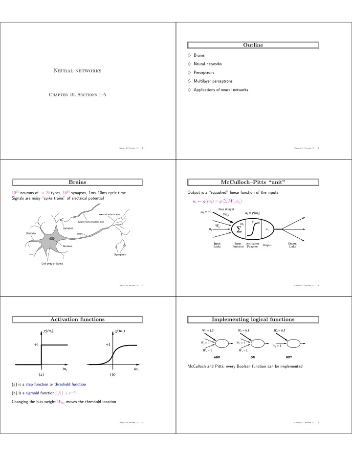
Outline ♦ Brains ♦ Neural networks Neural networks ♦ Perceptrons ♦ Multilayer perceptrons ♦ Applications of neural networks Chapter 19, Sections 1–5 Chapter 19, Sections 1–5 1 Chapter 19, Sections 1–5 2 Brains McCulloch–Pitts “unit” 10 11 neurons of > 20 types, 10 14 synapses, 1ms–10ms cycle time Output is a “squashed” linear function of the inputs: Signals are noisy “spike trains” of electrical potential a i ← g ( in i ) = g � Σ j W j,i a j � Bias Weight a 0 = − 1 a i = g ( in i ) W 0 ,i Axonal arborization g Axon from another cell in i W j,i Σ Synapse a j a i Dendrite Axon Input Input Activation Output Output Nucleus Links Function Function Links Synapses Cell body or Soma Chapter 19, Sections 1–5 3 Chapter 19, Sections 1–5 4 Activation functions Implementing logical functions g ( in i ) g ( in i ) W 0 = 1.5 W 0 = 0.5 W 0 = 0.5 W 1 = 1 W 1 = 1 + 1 + 1 W 1 = 1 W 2 = 1 W 2 = 1 AND OR NOT McCulloch and Pitts: every Boolean function can be implemented in i in i (a) (b) (a) is a step function or threshold function (b) is a sigmoid function 1 / (1 + e − x ) Changing the bias weight W 0 ,i moves the threshold location Chapter 19, Sections 1–5 5 Chapter 19, Sections 1–5 6

Network structures Feed-forward example Feed-forward networks: W 1,3 – single-layer perceptrons 1 3 W – multi-layer perceptrons 3,5 W 1,4 Feed-forward networks implement functions, have no internal state 5 Recurrent networks: – Hopfield networks have symmetric weights ( W i,j = W j,i ) W W 2,3 g ( x ) = sign ( x ) , a i = ± 1 ; holographic associative memory 4,5 2 4 – Boltzmann machines use stochastic activation functions, W 2,4 ≈ MCMC in BNs – recurrent neural nets have directed cycles with delays Feed-forward network = a parameterized family of nonlinear functions: have internal state (like flip-flops), can oscillate etc. ⇒ a 5 = g ( W 3 , 5 · a 3 + W 4 , 5 · a 4 ) = g ( W 3 , 5 · g ( W 1 , 3 · a 1 + W 2 , 3 · a 2 ) + W 4 , 5 · g ( W 1 , 4 · a 1 + W 2 , 4 · a 2 )) Chapter 19, Sections 1–5 7 Chapter 19, Sections 1–5 8 Perceptrons Expressiveness of perceptrons Consider a perceptron with g = step function (Rosenblatt, 1957, 1960) Can represent AND, OR, NOT, majority, etc. Represents a linear separator in input space: Σ j W j x j > 0 or W · x > 0 Perceptron output 1 I I I 0.9 1 1 1 0.8 0.7 0.6 0.5 1 1 1 0.4 0.3 0.2 -4 -2 0 2 4 0.1 Output Input 0 W j,i ? -4 x 2 Units Units -2 0 2 x 1 4 0 0 0 I I I 0 1 0 1 0 1 2 2 2 I I I I I xor I (a) and (b) or (c) 1 2 1 2 1 2 Chapter 19, Sections 1–5 9 Chapter 19, Sections 1–5 10 Perceptron learning Perceptron learning contd. Learn by adjusting weights to reduce error on training set Perceptron learning rule converges to a consistent function for any linearly separable data set The squared error for an example with input x and true output y is E = 1 2 Err 2 ≡ 1 1 1 2( y − h W ( x )) 2 , Proportion correct on test set Proportion correct on test set 0.9 0.9 Perform optimization search by gradient descent: 0.8 0.8 Decision tree Perceptron 0.7 0.7 ∂E = Err × ∂ Err ∂ y − g ( Σ n � � = Err × j = 0 W j x j ) 0.6 Perceptron 0.6 ∂W j ∂W j ∂W j Decision tree 0.5 0.5 = − Err × g ′ ( in ) × x j 0.4 0.4 0 10 20 30 40 50 60 70 80 90 100 0 10 20 30 40 50 60 70 80 90 100 Simple weight update rule: Training set size Training set size W j ← W j + α × Err × g ′ ( in ) × x j E.g., +ve error ⇒ increase network output ⇒ increase weights on +ve inputs, decrease on -ve inputs Chapter 19, Sections 1–5 11 Chapter 19, Sections 1–5 12

Multilayer perceptrons Expressiveness of MLPs Layers are usually fully connected; All continuous functions w/ 2 layers, all functions w/ 3 layers numbers of hidden units typically chosen by hand Output units a i h W ( x 1 , x 2 ) h W ( x 1 , x 2 ) 0.9 1 W j,i 0.9 0.8 0.8 0.7 0.7 0.6 0.6 0.5 0.5 0.4 0.4 0.3 Hidden units 0.3 a j 0.2 0.2 0.1 -4 -2 0 2 4 -4 -2 0 2 4 0.1 0 0 x 2 x 2 -4 -4 -2 -2 0 0 2 2 x 1 x 1 4 4 W k,j Input units a k Chapter 19, Sections 1–5 13 Chapter 19, Sections 1–5 14 Back-propagation learning Back-propagation derivation Output layer: same as for single-layer perceptron, The squared error on a single example is defined as E = 1 i ( y i − a i ) 2 , W j,i ← W j,i + α × a j × ∆ i � 2 where ∆ i = Err i × g ′ ( in i ) where the sum is over the nodes in the output layer. Hidden layer: back-propagate the error from the output layer: ∂E = − ( y i − a i ) ∂a i = − ( y i − a i ) ∂g ( in i ) ∂W j,i ∂W j,i ∂W j,i ∆ j = g ′ ( in j ) i W j,i ∆ i . � = − ( y i − a i ) g ′ ( in i ) ∂ in i ∂   = − ( y i − a i ) g ′ ( in i ) j W j,i a j �   Update rule for weights in hidden layer: ∂W j,i ∂W j,i   = − ( y i − a i ) g ′ ( in i ) a j = − a j ∆ i W k,j ← W k,j + α × a k × ∆ j . (Most neuroscientists deny that back-propagation occurs in the brain) Chapter 19, Sections 1–5 15 Chapter 19, Sections 1–5 16 Back-propagation derivation contd. Back-propagation learning contd. At each epoch, sum gradient updates for all examples and apply ∂E i ( y i − a i ) ∂a i i ( y i − a i ) ∂g ( in i ) = − = − � � ∂W k,j ∂W k,j ∂W k,j 14 i ( y i − a i ) g ′ ( in i ) ∂ in i ∂   = − = − i ∆ i j W j,i a j 12 � � �   Total error on training set   ∂W k,j ∂W k,j 10 ∂a j ∂g ( in j ) = − i ∆ i W j,i = − i ∆ i W j,i � � 8 ∂W k,j ∂W k,j 6 i ∆ i W j,i g ′ ( in j ) ∂ in j = − � ∂W k,j 4 ∂   2 = − i ∆ i W j,i g ′ ( in j ) k W k,j a k � �     ∂W k,j 0 i ∆ i W j,i g ′ ( in j ) a k = − a k ∆ j 0 50 100 150 200 250 300 350 400 = − � Number of epochs Usual problems with slow convergence, local minima Chapter 19, Sections 1–5 17 Chapter 19, Sections 1–5 18

Back-propagation learning contd. Handwritten digit recognition 1 0.9 % correct on test set 0.8 0.7 3-nearest-neighbor = 2.4% error 0.6 Multilayer network 400–300–10 unit MLP = 1.6% error Decision tree LeNet: 768–192–30–10 unit MLP = 0.9% 0.5 0.4 0 10 20 30 40 50 60 70 80 90 100 Training set size Chapter 19, Sections 1–5 19 Chapter 19, Sections 1–5 20 Summary Most brains have lots of neurons; each neuron ≈ linear–threshold unit (?) Perceptrons (one-layer networks) insufficiently expressive Multi-layer networks are sufficiently expressive; can be trained by gradient descent, i.e., error back-propagation Many applications: speech, driving, handwriting, credit cards, etc. Chapter 19, Sections 1–5 21