Survival analysis in R Niels Richard Hansen This note describes a - - PDF document

Survival analysis in R

Niels Richard Hansen This note describes a few elementary aspects of practical analysis of survival data in R. For further information we refer to the book “Introductory Statistics with R” by Peter Dalgaard and “Dynamic Regression Models for Survival Data” by Torben Martinussen and Thomas Scheike and to the R help files. There is also the classical reference “Statistical Models Based on Counting Processes” by Andersen, Borgan, Gill and Keiding. The analyses that we will do can all be done using the functions in library sur-

• vival. That library also contains some example data sets.

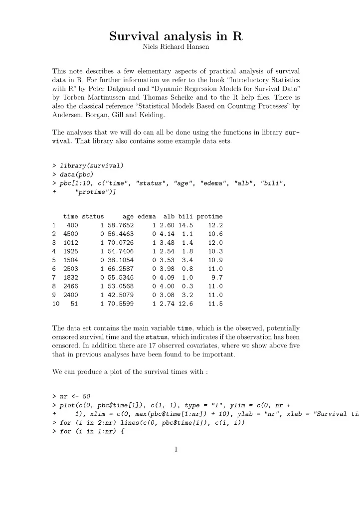
> library(survival) > data(pbc) > pbc[1:10, c("time", "status", "age", "edema", "alb", "bili", + "protime")] time status age edema alb bili protime 1 400 1 58.7652 1 2.60 14.5 12.2 2 4500 0 56.4463 0 4.14 1.1 10.6 3 1012 1 70.0726 1 3.48 1.4 12.0 4 1925 1 54.7406 1 2.54 1.8 10.3 5 1504 0 38.1054 0 3.53 3.4 10.9 6 2503 1 66.2587 0 3.98 0.8 11.0 7 1832 0 55.5346 0 4.09 1.0 9.7 8 2466 1 53.0568 0 4.00 0.3 11.0 9 2400 1 42.5079 0 3.08 3.2 11.0 10 51 1 70.5599 1 2.74 12.6 11.5 The data set contains the main variable time, which is the observed, potentially censored survival time and the status, which indicates if the observation has been

• censored. In addition there are 17 observed covariates, where we show above five

that in previous analyses have been found to be important. We can produce a plot of the survival times with : > nr <- 50 > plot(c(0, pbc$time[1]), c(1, 1), type = "l", ylim = c(0, nr + + 1), xlim = c(0, max(pbc$time[1:nr]) + 10), ylab = "nr", xlab = "Survival tim > for (i in 2:nr) lines(c(0, pbc$time[i]), c(i, i)) > for (i in 1:nr) { 1

+ if (pbc$status[i] == 0) + points(pbc$time[i], i, col = "red", pch = 20) + if (pbc$status[i] == 1) + points(pbc$time[i], i) + }

1000 2000 3000 4000 10 20 30 40 50 Survival time nr

Estimation of the survival function using the Kaplan-Meier estimator can be done using the survfit function. > pbc.surv <- survfit(Surv(pbc$time, pbc$status)) > pbc.surv Call: survfit(formula = Surv(pbc$time, pbc$status)) n events median 0.95LCL 0.95UCL 418 161 3395 3090 3853 > plot(pbc.surv) 2

1000 2000 3000 4000 0.0 0.2 0.4 0.6 0.8 1.0

The result from survfit is an R object of type survfit. Taking summary of a survfit object provides the non-parametric estimate of the survival function including additional information at a long list. The plot is perhaps more infor- mative with the added, pointwise confidence bands. The function Surv applied to the time and status variables for the PBC data is a function that create a survival object. A major point in a data set like the PBC data above is that we record covariate information on the individuals. It is no problem to split the estimation of the survival function according to a factor such as the binary edema variable in the PBC data. > pbc.surv <- survfit(Surv(pbc$time, pbc$status) ~ pbc$edema) > plot(pbc.surv, conf.int = TRUE, col = c("red", "blue")) 3

1000 2000 3000 4000 0.0 0.2 0.4 0.6 0.8 1.0

From the plot it seems clear that individuals without edema has a larger chance

• f a large survival time than those with edema. This can also be testet formally

with the so-called log-rank test. > survdiff(Surv(pbc$time, pbc$status) ~ pbc$edema) Call: survdiff(formula = Surv(pbc$time, pbc$status) ~ pbc$edema) N Observed Expected (O-E)^2/E (O-E)^2/V pbc$edema=0 368 121 151.0 5.94 96 pbc$edema=1 50 40 10.0 89.28 96 Chisq= 96

• n 1 degrees of freedom, p= 0

But what about including the other covariates also – especially the continuous

• nes? This can be handled in the framework of the Cox proportional hazards

model. > pbc.surv <- coxph(Surv(pbc$time, pbc$status) ~ pbc$edema) > summary(pbc.surv) 4

Call: coxph(formula = Surv(pbc$time, pbc$status) ~ pbc$edema) n= 418 coef exp(coef) se(coef) z p pbc$edema 1.63 5.09 0.185 8.82 0 exp(coef) exp(-coef) lower .95 upper .95 pbc$edema 5.09 0.197 3.54 7.3 Rsquare= 0.129 (max possible= 0.985 ) Likelihood ratio test= 57.7

• n 1 df,

p=3e-14 Wald test = 77.7

• n 1 df,

p=0 Score (logrank) test = 96

• n 1 df,

p=0 We can tell from the summary that the β corresponding to the covariate edema is significantly different from 0. We also see that the hazard rate for those with edema=1 is estimated as roughly 5 times the base-line hazard rate α0(t). We can include more covariates. > pbc.surv <- coxph(Surv(time, status) ~ edema + age + alb + bili + + protime, data = pbc) > summary(pbc.surv) Call: coxph(formula = Surv(time, status) ~ edema + age + alb + bili + protime, data = pbc) n= 418 coef exp(coef) se(coef) z p edema 0.7222 2.059 0.20764 3.48 5.1e-04 age 0.0365 1.037 0.00811 4.50 6.8e-06 alb

• 0.9266

0.396 0.20898 -4.43 9.2e-06 bili 0.1246 1.133 0.01271 9.80 0.0e+00 protime 0.1928 1.213 0.05770 3.34 8.3e-04 exp(coef) exp(-coef) lower .95 upper .95 edema 2.059 0.486 1.371 3.093 age 1.037 0.964 1.021 1.054 alb 0.396 2.526 0.263 0.596 bili 1.133 0.883 1.105 1.161 protime 1.213 0.825 1.083 1.358 5

Rsquare= 0.36 (max possible= 0.985 ) Likelihood ratio test= 186

• n 5 df,

p=0 Wald test = 218

• n 5 df,

p=0 Score (logrank) test = 309

• n 5 df,

p=0 It is of course also possible to transform the covariates before using them in the

• regression. For example;

> pbc.surv <- coxph(Surv(time, status) ~ edema + age + log(bili) + + log(alb) + log(protime), data = pbc) > summary(pbc.surv) Call: coxph(formula = Surv(time, status) ~ edema + age + log(bili) + log(alb) + log(protime), data = pbc) n= 418 coef exp(coef) se(coef) z p edema 0.6613 1.937 0.20595 3.21 1.3e-03 age 0.0382 1.039 0.00768 4.97 6.5e-07 log(bili) 0.8975 2.453 0.08271 10.85 0.0e+00 log(alb)

• 2.4524

0.086 0.65707 -3.73 1.9e-04 log(protime) 2.3458 10.442 0.77425 3.03 2.4e-03 exp(coef) exp(-coef) lower .95 upper .95 edema 1.937 0.5162 1.2938 2.901 age 1.039 0.9625 1.0234 1.055 log(bili) 2.453 0.4076 2.0863 2.885 log(alb) 0.086 11.6167 0.0237 0.312 log(protime) 10.442 0.0958 2.2895 47.624 Rsquare= 0.429 (max possible= 0.985 ) Likelihood ratio test= 234

• n 5 df,

p=0 Wald test = 233

• n 5 df,

p=0 Score (logrank) test = 297

• n 5 df,

p=0

A Theory

We consider n individuals, T ∗

1 , . . . , T ∗ n independent, positive random variables

(survival times). 6

Estimation of the distribution by the empirical distribution: ˆ F(t) = 1 n

n

• i=1

1(T ∗

i ≤ t)

and the survival function S(t) = 1 − F(t) ˆ S(t) = 1 − ˆ F(t) = 1 n

n

• i=1

1(T ∗

i > t).

Censoring by positive, random variables C1, . . . , Cn: We observe only Ti = min{T ∗

i , Ci}

and ∆i = 1(T ∗

i ≤ Ci).

Thus we observe the pairs (T1, ∆1), . . ., (Tn, ∆n). Define the counting process of deaths (non censored events) N(t) =

• i=1

1(Ti ≤ t, ∆i = 1). Define also the process of individuals at risk Y (t) =

n

• i=1

1(t ≤ Ti). The jumps for the counting process are given by the process ∆N(t) = N(t) − N(t−) = N(t) − lim

ǫ→0+ N(t − ǫ) ∈ {0, 1},

which is simply an indicator process for each jump (death). The Kaplan-Meier estimator of the survival function, based on censored survival times, is ˆ S(t) =

• s≤t
• 1 − ∆N(s)

Y (s)

• .

The factors are equal to 1 for all s where ∆N(s) = 0. If we denote by τi the time for the i’th jump, we can also write the estimator out as ˆ S(t) =

• 1 −

1 Y (τ1) 1 − 1 Y (τ2)

• . . .
• 1 −

1 Y (τN(t))

• Each factor can be interpreted as an estimator of the conditional probability of

dying in the time interval (τi, τi+1] given survival to time τi. 7

If F is continuous differentiable with derivative f (the density for the survival distribution then), we can introduce the hazard rate: α(t) = f(t) S(t). We see that α(t) = lim

ǫ→0+

1 ǫ F(t + ǫ) − F(t) S(t) = lim

ǫ→0+

1 ǫP(T ∗

i ∈ (t, t + ǫ] | T ∗ i > t).

Thus α(t) is the instantaneous rate of death at time t. The exponential distribution provides an example where α(t) = λ is constant. In general, we can always get back the the survival function from the hazard rate by S(t) = exp

• −

t

0 α(s)ds

• .

This means that we can specify a distribution via its hazard rate as well as its survival function. The Cox proportional hazards rate model is given as follows. We assume that we for each individual has a vector Xi = (X1i, . . . , Xmi)T of real valued covariates (they may be indicator variables as well). Then we specify the hazard rate for the i’th individual as αi(t, Xi) = α0(t) exp

 

m

• j=1

βjXij

  = α0(t) exp

• XTβ
• for an m-dimensional vector β of parameters.

The model is a semi-parametric model. The estimation of α0(t) has secundary interest whereas the estimation of the β’s is of primary interest. We see that αi(t, Xi) αi(t, Xi + (0, . . ., 0, δ, 0, . . ., 0)T = e−δβj if the δ above is at the j’th position in the vector. This gives an interpretation of the parameters as the log-relative risks for a given covariate. The parameters are estimated by solving the estimation equation

n

• i=1

(Xi − E(β, Ti))∆i = 0 where E(β, Ti) =

• i 1(t ≤ Ti)Xi exp(XT

i β)

• i 1(t ≤ Ti) exp(XT

i β) .

8