Supporting Information for Phytoplankton blooms at 1 increasing - - PDF document

Supporting Information for ’Phytoplankton blooms at

1

increasing levels of atmospheric carbon dioxide:

2

experimental evidence for negative effects on

3

prymnesiophytes and positive on small

4

picoeukaryotes’

5

S-3 Methods

6

S-3.1 pH dye preparation, measurements and corrections

7

Determination of seawater pH followed in principle the spectrophotometrical approach of

8

Clayton and Byrne (1993) described in Dickson, A. G. and Sabine, C. L. and Christian, J.R.

9

(Eds.) (2007) making use of the dye m-cresol purple (Acros Organics, CAS 62625-31-4, Lot

10

A026431) at 25◦C in a 10 cm thermostated cuvette on a Cary 100 (Varian). Concerning the

11

dye, 300 ml of an about 2 mM solution was prepared in Milli-Q, the ionic strength brought to

12

0.66 with NaCl (matching that of seawater with a salinity of ∼32) and the pHT (pH on the

13

total scale) adjusted to about 7.6 (at 25◦C). After that the solution was sterile filtered (0.2 µm)

14

into a gas and light impermeable sampling bag (Supelco), filled without air.

15

For measurements, 5 ml of sample water was pumped from the bottom of a 100 ml bottle,

16

brought to 25◦C in a thermostated water bath, into a 25 ml syringe pump (Tecan, Cavro XLP

17

6000), followed by about 50 µl of m-cresol purple dye solution, and then mixed within the

18

syringe with an additional 15 ml of sample water. This mixture was then injected into the

19

10 cm flow-through cuvette (with a capacity of about 8 ml), which had been previously filled

20

1

carefully whiteout air bubbles with filtered (0.2 µm) fjord water, or already contained sample

21

• water. Samples were measured from low to high fCO2, and potential carry-over from a previ-

22

• us sample was usually below detection limit. Each seawater sample was measured in triplic-

23

ates and precision of replicate measurements was typically 0.001 or better for the higher and

24

0.002 or better for the lower pH treatments (with the threshold at an in situ pH of about 7.700).

25

Measured absorption spectra (780 to 380 nm at 1nm resolution and a scan rate of 600 nm per

26

minute) were corrected for tiny air bubble entrainment by comparison to an absorption mean

27

between 735 and 725 nm, wavelengths at which the dye is non-absorbent, of a baseline in

28

Milli-Q. The resulting absorption ratio at 578 and 434 nm was then used to calculate pHT us-

29

ing the acid dissociation constant and extinction coefficient ratios of m-cresol purple reported

30

in Dickson, A. G. and Sabine, C. L. and Christian, J.R. (Eds.) (2007). Furthermore, absorb-

31

ance at 578 nm, the isosbestic point, was used to correct the calculated pH by accounting for

32

inevitable changes due to dye addition (about -0.005 pH units at the highest and +0.014 at

33

the lowest pH), similar to the method described in Clayton and Byrne (1993). For that pur-

34

pose five seawater batches of different pH, one liter each, covering the entire measurement

35

range, were prepared, and in each pH was determined as described above, but with increasing

36

amounts of dye (six levels). At each pH level a linear correlation between the change in pH in

37

relation to the absorbance at the isosbestic point (a measure for the amount of dye added) was

38

• constructed. The combination of all six correlations at each pH level then led to an uniform

39

linear relation describing the change in measured pH in response to a certain amount of dye

40

added at a certain pH.

41

To assess the accuracy of pH measurements, and to account for potential impurities in the

42

m-cresol purple sodium salt, pHT was measured and corrected as described above on five

43

replicates of CRM batch 108 (freshly opened). However, no further corrections were applied

44

2

as measured pHT (7.8791±0.0002) was off less then 0.001 units the theoretical one of 7.8786,

45

calculated from known DIC (2022.7 µmol kg−1), total alkalinity, TA (2218.0 µmol kg−1),

46

salinity (33.224), phosphate (0.41 µmol kg−1) and silicate (2.9 µmol kg−1) concentrations

47

using the dissociation constants for carbonic acid from Mehrbach et al. (1973) as refitted by

48

Lueker et al. (2000).

49

S-3.2 pH sample filtration

50

Prior to analysis samples for pH were transferred from the 500 ml glass stoppered bottles

51

(Schott Duran) with a membrane pump to 100 ml glass stoppered bottles (Schott Duran) at a

52

flow rate of about 50 ml per minute, passing a sterile 0.2 µm filter (Sarstedt Filtropur, PES

53

membrane). For that the sample water was pumped from the bottom of the 500 ml bottles,

54

filling the 100 ml bottles through a serological needle from bottom to top with about 100 ml

55

• f additional overflow. Since about 300 ml of sample water always remained in the larger

56

bottles, tubing was Tygon and the smaller bottles were filled from bottom to top with consider-

57

able overflow, potential CO2 gas exchange with the atmosphere, impacting seawater pH, was

58

• minimized. Filtration removed all particulate organic matter which, at relatively high concen-

59

trations, can influence the precision of spectrophotometric measurements. Furthermore, the

60

close to sterile seawater samples are relatively stable as potential biological activity by phyto-

61

plankton or bacteria, otherwise impacting pH, is minimized. The 100 ml bottles were closed

62

without headspace and, if not measured within the next couple of hours, stored at 4◦C in the

63

dark.

64

3

S-3.3 Carbonate chemistry calculations

65

In a first step measured pHT (at 25◦C) and DIC was used to calculate practical alkalinity (PA).

66

The second step involved calculating pHT and all the other carbonate chemistry components

67

such as the fugacity of carbon dioxide, fCO2, at in-situ temperature and salinity conditions

68

from measured DIC and calculated PA, using the dissociation constants for carbonic acid

69

from Mehrbach et al. (1973) as refitted by Lueker et al. (2000). Since there were no DIC and

70

spectrophotometric pH measurements on the first three (t-3 to t-1) and last six days (28 to 34),

71

carbonate chemistry speciation had to be estimated using CTD-derived mean water column

72

pH measurements, brought to the total scale with CTD to spectrophotometric pH relations

73

for day 0 and 27 (compare section 3.5), and salinity based estimates of PA. For that purpose,

74

mean water column salinity changes were considered a proxy for changes in PA, taking a mean

75

initial PA of 2180 µmol kg−1 and a mean initial salinity of 31.95. The assumption that the

76

sole drivers of TA changes are freshwater input by rain and evaporation obviously ignores the

77

impact of phosphate and nitrate assimilation and calcium carbonate production on TA. Never-

78

theless, here estimates of carbonate chemistry speciation will hardly be affected as 1) changes

79

in alkalinity due to nutrient assimilation (about +5 µmol kg−1) and calcification (maximum

80

• f -2 µmol kg−1), which furthermore work in opposite directions, were smaller than those by

81

freshwater input (about -9 µmol kg−1) and 2) the estimates are based on measured pH, ren-

82

dering the carbonate system practically insensitive to even relatively large PA uncertainties

83

(depending on actual CO2 level, 10 µmol kg−1 correspond to only a few µatm).

84

4

S-4 Results

85

S-4.1 Changes in light, salinity and temperature

86

Average incident photosynthetic active radiation (PAR) measured in air was similar during all

87

phases, although slightly higher during the first two weeks (Fig. S-3). Light profiles taken

88

within and outside the mesocosms were generally very similar, with marginally higher atten-

89

uation in the upper 10 m of the mesocosms, possibly due to shading by the floating structures,

90

and potentially higher particulate biomass (Fig. S-3b). Nevertheless, no significant differ-

91

ences were observed between mesocosms and through time (data not shown), while attenu-

92

ation coefficients were similar in comparison to a previous KOSMOS study, with typical kd

93

values between 0.3 and 0.4 (Schulz et al., 2013). Using an average incident PAR intensity

94

• f 450 µmol m−2s−1 during daylight, depth-averaged (0.3-23 m) light conditions were about

95

56 µmol m−2s−1. This is probably at least three times lower then in two previous mesocosm

96

experiments at the same location in bags of only 5 (Engel et al., 2005) and 10 meters depth

97

Schulz et al. (2008).

98

Depth-averaged salinity in the fjord ranged from 30.20 to 31.54, thus being more variable

99

than in the mesocosms (Fig. S-2a). Ignoring the initial salt addition for volume determinations,

100

depth-integrated variability within the mesocosms was about 0.15 salinity units, and while

101

being relatively stable throughout the first 2 weeks, constantly decreased towards the end of

102

the experiment. This decrease was most likely due to rain water input as most pronounced

103

in the upper 5-10 m of the mesocosms (Fig. S-2b). Overall dilution by rainwater was on the

104

• rder of 5.

105

Average water column temperatures steadily increased within the mesocosms and the fjord,

106

from initially about 7 to 10◦C half way through the experiment (Fig S-2c). Although surface

107

5

waters continued to warm, upwelling of colder deeper waters in the fjord to up to 15 m depth,

108

also mirrored in salinity changes (Fig S-2a), kept average temperatures relatively constant

109

until the end of the experiment. Average temperatures did not significantly exceed 10◦C, and

110

reached up to 13◦C in the upper meter by the end of the experiment Fig S-2c).

111

6

References

112

Clayton, T. D. and Byrne, R. H. (1993). Spectrophotometric seawater pH measurements: total

113

hydrogen ion concentration scale calibrations of m-cresol purple and at-sea results. Deep-

114

Sea Res. 40, 2115–2129

115

Dickson, A. G. and Sabine, C. L. and Christian, J.R. (Eds.) (2007). Guide to Best Practices for

116

Ocean CO2 Measurements. PICES Special Publication 3

117

Engel, A., Zondervan, I., Aerts, K., Beaufort, L., Benthien, A., Chou, L., et al. (2005). Testing

118

the direct effect of CO2 concentration on a bloom of the coccolithophorid Emiliania huxleyi

119

in mesocosm experiments. Limnol. Oceanogr. 50, 493–507

120

Lueker, T. J., Dickson, A. G., and Keeling, C. D. (2000). Ocean pCO2 calculated from dissolved

121

inorganic carbon, alkalinity, and equations for K1 and K2: validation based on laboratory

122

measurements of CO2 in gas and seawater at equilibrium . Mar. Chem. 70, 105–119

123

Mehrbach, C., Culberson, C. H., Hawley, J. E., and Pytkowicz, R. M. (1973). Measurements

124

• f the apparent dissociation constants of carbonic acid in seawater at atmospheric pressure.

125

• Limnol. Oceanogr. 18, 897–907

126

Schulz, K. G., Bellerby, R. G. J., Brussaard, C. P. D., B¨ udenebnder, J., Czerny, J., Engel, A., et al.

127

(2013). Temporal biomass dynamics of an Arctic plankton bloom in response to increasing

128

levels of atmospheric carbon dioxide. Biogeosci. 10, 161–180

129

Schulz, K. G., Riebesell, U., Bellerby, R. G. J., Biswas, H., Meyer¨

• fer, M., M¨

uller, M. N., et al.

130

(2008). Build-up and decline of organic matter during PeECE III. Biogeosci. 5, 707–718

131

7

Table S-1: R2, F and p values for statistically significant correlations (p < 0.05) between the mean of a measurement parameter and fCO2 during a certain phase of the experiment. For details see section 3.8. Positive correlations are shown in bold, negative in italic (in total 60 out of 160). Superscripts a, b, c, d, and frefer to data shown in Figs. 3, S-5, 4, 5, S-6, respectively Phase I Phase II Phase III Phase IV

• adj. R2

F p

• adj. R2

F p

• adj. R2

F p

• adj. R2

F p

a,dChla

0.7598 23.14 0.003 0.6734 15.43 0.008

bPOC

0.7002 15.02 0.012

bPON

0.5120 8.34 0.028

bPOP

0.7583 22.96 0.003 0.7561 22.70 0.003

bBSi bDOC

0.5041 8.12 0.029

bDON bDOP

0.5268 8.79 0.025 0.5260 8.77 0.025

aNitrate

0.4199 6.07 0.049

aAmmonia

0.7633 23.57 0.003 0.8037 29.66 0.002

aPhosphate

0.5579 9.835 0.020

aSilicate a∆[O2]

0.6027 11.62 0.014 0.7360 20.51 0.004 8

• Tab. continued

Phase I Phase II Phase III Phase IV

• adj. R2

F p

• adj. R2

F p

• adj. R2

F p

• adj. R2

F p

cChlaHapto

0.8215 33.23 0.001 0.4451 6.62 0.042 0.8032 29.56 0.002

cChlaChryso

0.5287 8.85 0.025

cChlaDino cChlaDiatom

0.6998 17.31 0.006

cChlaChloro

0.9055 68.06 <0.001 0.8454 39.27 <0.001 0.6656 14.93 0.008 0.5238 8.70 0.026

cChlaCrypto

0.7646 23.74 0.003

cChlaCyano

0.4613 6.99 0.038 0.7739 24.97 0.003 0.9391 108.9 <0.001 0.7984 28.73 0.002

dSynFCM

0.5633 10.03 0.019 0.4820 7.52 0.034 0.9212 82.81 <0.001 0.7292 19.85 0.004

dPicoFCM

0.8590 43.63 <0.001 0.9560 153.15 <0.001 0.8948 60.56 <0.001 0.6879 16.43 0.007

dEhuxFCM

0.6805 15.92 0.007 0.4631 7.04 0.038 0.4412 6.53 0.043

dNano smallFCM

0.5137 8.39 0.030

dNano bigFCM

0.5936 11.23 0.015 0.8702 47.93 < 0.001

dCryptoFCM

0.6614 14.67 0.009

eHaptoMicro

0.6952 16.96 0.006 0.5874 10.96 0.016 n.a. n.a. n.a.

eDino NTMicro

0.6366 13.26 0.011 n.a. n.a. n.a.

eDino TMicro

n.a. n.a. n.a.

fDiatomMicro

0.7707 24.52 0.003 n.a. n.a. n.a.

eChloroMicro

0.6246 12.65 0.012 n.a. n.a. n.a.

eCryptoMicro

n.a. n.a. n.a.

eDino HTMicro

0.5171 8.50 0.027 n.a. n.a. n.a.

• eTot. autoMicro

0.8422 36.36 < 0.001 n.a. n.a. n.a. 9

Figure S-1: Schematic drawing of a KOSMOS mesocosm deployed in Raunefjorden, Nor-

• way. The orange flanges at depth connect the funnel-shaped sediment trap to the

rest of the bag. 10

−25 −20 −15 −10 −5

31.619 31.65 31.661 32.002 32.014 32.026 32.021 32.011 32.011 32.013 32.012 32.006 32.013 32.015 32.015 32.003 32.015 32.014 32.004 31.989 31.988 31.991 31.983 31.98 31.971 31.959 31.962 31.951 31.905 31.898 31.901 31.91 31.916 31.897 31.895 31.89 31.895

b

Depth (m) 31.6 31.8 32 32.2 32.4 32.6 −50 −40 −30 −20 −10

31.375 31.54 31.503 31.125 31.055 30.636 30.782 30.71 30.601 30.594 30.595 30.723 30.849 31.023 31.062 30.903 30.946 30.644 30.451 30.579 30.763 30.881 30.799 30.683 30.373 30.384 30.399 30.723 30.512 30.511 30.702 31.273 31.295 30.947 30.567 30.204 30.407

a

30 31 32 33 34 35 10 20 30 −25 −20 −15 −10 −5

6.85 6.99 6.98 7.36 7.98 8.63 8.71 8.86 9.16 9.53 9.65 9.61 9.45 9.27 9.07 9.53 9.63 9.85 10 9.88 9.72 9.54 9.56 9.53 9.71 9.82 9.87 9.58 9.72 9.8 9.89 9.48 9.27 9.47 9.8 10 10.1

c

Days 6 8 10 12

Figure S-2: Vertical distribution and dynamics of salinity measured in the fjord (a) and meso- cosm M9 (b) together with those of temperature (c), given in degrees Celsius. Note that with the exception of mesocosm M2 which had a hole right from the beginning, allowing fjord and mesocosm water to exchange, temperature and sa- linity dynamics in all other mesocosms were practically identical. Numbers rep- resent depth-averaged (0.3-23 m) values. 11

5 10 15 20 25 30 35 500 1000 1500 2000 2500 Days PAR (µmol m−2 s−1)

I II III IV

721 551 362 407 443

a

0.2 0.4 0.6 0.8 1 −25 −20 −15 −10 −5 relative PAR Depth (m)

b

Turbidity (kg m

−3)

Figure S-3: (a) Changes in photosynthetic active radiation (PAR) in air, and (b) a typical ver- tical light (black) and turbidity (grey) profile in a mesocosm (solid lines) and the fjord (dotted lines). Numbers in (a) denote average daily PAR levels during a cer- tain phase, indicated by vertical lines and Roman numbers. In (b) the vertical line marks the 10% level of incident light. For details on measurements see section 3.5. 12

−25 −20 −15 −10 −5

M1

8.11 8.09 8.07 8.09 8.12 7.97 7.8 7.75 7.76 7.72 7.7 7.73 7.76 7.76 NaN 7.75 7.78 7.79 7.78 7.78 7.81 7.81 7.84 7.86 7.86 7.85 7.86 7.87 7.87 7.85 7.86 7.87 7.87 7.89 7.87 7.87 7.88 8.16 8.1 8.06 8.08 8.11 7.96 7.78 7.74 7.77 7.73 7.72 7.77 7.79 7.79 7.82 7.81 7.82 7.82 7.82 7.85 7.91 7.93 7.95 7.95 7.96 7.95 7.97 7.96 7.95 7.94 7.94 7.97 7.97 8 7.99 7.98 7.99 8.06 8.07 8.07 8.09 8.12 8 7.83 7.76 7.76 7.71 7.69 7.7 7.73 7.73 NaN 7.71 7.75 7.75 7.75 7.75 7.76 7.75 7.76 7.78 7.77 7.76 7.78 7.79 7.81 7.79 7.8 7.81 7.81 7.81 7.8 7.8 7.79

Depth (m) −25 −20 −15 −10 −5

M2

8.11 8.1 8.07 8.09 8.13 8.12 8.13 8.14 8.13 8.13 8.13 8.12 8.13 8.14 8.13 8.12 8.12 8.14 8.11 8.12 8.12 8.12 8.15 8.15 8.15 8.15 8.15 8.15 8.14 8.15 8.14 8.15 8.13 8.14 8.15 8.13 NaN 8.15 8.11 8.06 8.08 8.13 8.13 8.14 8.15 8.15 8.15 8.15 8.14 8.14 8.16 8.15 8.15 8.13 8.16 8.13 8.14 8.15 8.17 8.2 8.2 8.2 8.2 8.2 8.19 8.18 8.19 8.17 8.21 8.17 8.19 8.2 8.19 NaN 8.07 8.07 8.07 8.08 8.13 8.11 8.12 8.12 8.11 8.11 8.1 8.1 8.11 8.12 8.12 8.1 8.1 8.11 8.1 8.11 8.1 8.1 8.11 8.11 8.1 8.1 8.11 8.11 8.11 8.11 8.1 8.11 8.09 8.11 8.11 8.09 NaN

M3

8.12 8.1 8.08 8.06 8.12 7.98 7.8 7.68 7.69 7.61 7.62 7.62 7.66 7.65 7.66 7.65 7.67 7.68 7.69 7.71 7.73 7.73 7.75 7.78 7.77 7.78 7.8 7.81 7.81 7.82 7.81 7.8 7.78 7.79 7.81 7.79 7.79 8.16 8.12 8.07 8.06 8.12 7.97 7.78 7.66 7.69 7.61 7.64 7.67 7.7 7.69 7.72 7.73 7.72 7.73 7.75 7.81 7.84 7.86 7.87 7.88 7.9 7.92 7.94 7.94 7.93 7.92 7.94 7.95 7.92 7.95 7.95 7.93 7.94 8.07 8.08 8.09 8.06 8.12 7.99 7.84 7.7 7.69 7.61 7.6 7.6 7.63 7.62 7.62 7.61 7.62 7.63 7.66 7.66 7.67 7.65 7.67 7.69 7.67 7.67 7.69 7.72 7.73 7.76 7.72 7.71 7.7 7.7 7.71 7.69 7.69

M4

8.09 8.07 8.06 8.06 8.13 8.1 8.11 8.13 8.12 8.12 8.12 8.12 8.12 8.14 8.13 8.12 8.12 8.11 8.1 8.13 8.11 8.13 8.13 8.13 8.13 8.14 8.15 8.15 8.14 8.13 8.14 8.15 8.13 8.14 8.14 8.13 8.13 8.15 8.08 8.05 8.06 8.13 8.1 8.12 8.14 8.14 8.14 8.15 8.14 8.13 8.15 8.14 8.14 8.12 8.12 8.1 8.14 8.12 8.16 8.17 8.16 8.18 8.18 8.2 8.19 8.18 8.18 8.17 8.19 8.15 8.18 8.17 8.16 8.17 8.05 8.06 8.06 8.07 8.13 8.09 8.1 8.11 8.1 8.1 8.1 8.1 8.1 8.12 8.12 8.11 8.11 8.1 8.09 8.12 8.1 8.12 8.11 8.1 8.1 8.11 8.12 8.12 8.11 8.11 8.11 8.12 8.1 8.11 8.11 8.1 8.1

M5

8.1 8.08 8.06 8.05 8.11 7.97 7.8 7.63 7.56 7.51 7.54 7.55 7.59 7.58 7.6 7.6 7.62 7.62 7.64 7.68 7.68 7.69 7.7 7.72 7.71 7.72 7.74 7.75 7.77 7.74 7.75 7.77 7.75 7.77 7.76 7.75 7.76 8.16 8.1 8.05 8.05 8.11 7.96 7.77 7.6 7.55 7.52 7.56 7.62 7.65 7.64 7.67 7.72 7.69 7.7 7.73 7.82 7.83 7.85 7.85 7.84 7.87 7.9 7.93 7.93 7.93 7.92 7.92 7.96 7.93 7.95 7.94 7.92 7.94 8.05 8.05 8.06 8.06 8.12 7.98 7.84 7.66 7.58 7.52 NaN 7.52 7.55 7.54 7.55 7.54 7.56 7.55 7.59 7.62 7.6 7.6 7.61 7.63 7.6 7.6 7.62 7.63 7.66 7.63 7.64 7.65 7.64 7.65 7.64 7.63 7.64

M6

8.09 8.07 8.06 8.05 8.12 8.05 8.06 8.07 8.07 8.03 8.03 8.03 8.04 8.04 8.05 8.04 8.03 8.01 8.02 8.05 8.04 8.06 8.06 8.06 8.07 8.07 8.07 8.09 8.08 8.07 8.08 8.09 8.07 8.08 8.07 8.06 8.07 8.13 8.07 8.04 8.05 8.12 8.04 8.07 8.08 8.08 8.03 8.04 8.04 8.05 8.05 8.06 8.06 8.04 8.03 8.03 8.06 8.07 8.11 8.11 8.1 8.12 8.12 8.12 8.13 8.11 8.11 8.11 8.14 8.12 8.14 8.13 8.12 8.12 8.04 8.07 8.06 8.05 8.12 8.05 8.06 8.06 8.05 8.02 8.02 8.02 8.03 8.04 8.04 8.03 8.02 8 8.01 8.04 8.03 8.04 8.03 8.03 8.03 8.02 8.04 8.06 8.05 8.04 8.05 8.05 8.04 8.04 8.03 8.02 8.02

M7

8.09 8.08 8.05 8.06 8.13 7.99 7.84 7.59 7.41 7.36 7.38 7.4 7.44 7.43 7.46 7.45 7.49 7.5 7.52 7.56 7.57 7.57 7.62 7.63 7.63 7.64 7.65 7.65 7.68 7.65 7.66 7.67 7.66 7.65 7.66 7.64 7.65 8.14 8.1 8.05 8.06 8.13 7.98 7.83 7.58 7.4 7.38 7.41 7.48 7.5 7.51 7.53 7.57 7.56 7.57 7.62 7.73 7.76 7.78 7.81 7.78 7.82 7.83 7.83 7.82 7.84 7.83 7.84 7.88 7.85 7.83 7.84 7.82 7.85 8.04 8.06 8.05 8.06 8.13 8 7.86 7.6 7.42 7.37 7.38 7.37 7.4 7.39 7.41 7.39 7.42 7.43 7.47 7.48 7.47 7.47 7.5 7.51 7.5 7.5 7.51 7.53 7.56 7.52 7.55 7.54 7.55 7.54 7.54 7.52 7.53

M8

8.1 8.08 8.05 8.06 8.12 7.97 7.87 7.89 7.88 7.87 7.87 7.88 7.88 7.9 7.89 7.89 7.89 7.88 7.89 7.9 7.9 7.93 7.94 7.95 7.95 7.96 7.97 7.96 7.98 7.95 7.96 7.99 7.97 7.97 7.97 7.95 7.93 8.15 8.1 8.05 8.05 8.12 7.97 7.86 7.89 7.89 7.88 7.89 7.9 7.9 7.92 7.92 7.92 7.9 7.91 7.93 7.95 7.97 8.03 8.03 8.03 8.05 8.04 8.05 8.04 8.05 8.03 8.04 8.07 8.05 8.06 8.05 8.03 7.92 8.04 8.05 8.06 8.06 8.12 7.99 7.89 7.89 7.88 7.86 7.86 7.86 7.86 7.88 7.86 7.87 7.87 7.86 7.87 7.88 7.87 7.89 7.88 7.89 7.88 7.88 7.9 7.9 7.92 7.89 7.91 7.92 7.91 7.92 7.91 7.89 7.94

10 20 30 −25 −20 −15 −10 −5

M9

8.1 8.08 8.07 8.05 8.12 7.97 7.8 7.42 7.21 7.2 7.22 7.25 7.29 7.29 7.32 7.32 7.35 7.36 7.4 7.44 7.46 7.48 7.47 7.52 7.49 7.51 7.53 7.54 7.57 7.53 7.55 7.57 7.54 7.55 7.53 7.53 7.55 8.15 8.09 8.06 8.04 8.12 7.97 7.77 7.41 7.22 7.23 7.28 7.37 7.39 7.4 7.43 7.49 7.43 7.46 7.55 7.67 7.72 7.75 7.7 7.69 7.7 7.73 7.77 7.75 7.78 7.76 7.78 7.84 7.8 7.79 7.77 7.77 7.81 8.05 8.06 8.07 8.05 8.12 7.97 7.83 7.45 7.22 7.19 7.19 7.19 7.23 7.22 7.25 7.23 7.27 7.27 7.33 7.33 7.34 7.34 7.33 7.38 7.35 7.35 7.38 7.39 7.44 7.39 7.41 7.41 7.4 7.4 7.39 7.39 7.39

Days 10 20 30 −50 −40 −30 −20 −10

Fjord

8.1 8.1 8.09 8.15 8.18 8.17 8.17 8.17 8.18 8.18 8.15 8.16 8.16 8.17 8.17 8.17 8.16 8.16 8.16 8.12 8.15 8.13 8.15 8.15 8.16 8.15 8.13 8.14 8.14 8.15 8.13 8.09 8.06 8.09 8.1 8.11 8.1

Days 7.2 7.4 7.6 7.8 8 8.2

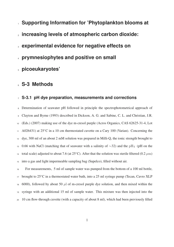
Figure S-4: Temporal development of pH (corrected to the total scale) in the mesocosms and the fjord as measured by a hand-operated CTD. Numbers at -5, -11 and -19 m depth denote daily averages representative for 0.3-5 m, 0.3-23 m and 15-23 m,

• respectively. For details on pH corrections applied see section 3.5.

13

10 15 20 25 30 I II III IV

a

1 2 3 4 5 6

b

0.1 0.2 0.3 c 5 10 15 20 25 30 35 0.2 0.4 0.6 0.8 Days

d

80 100 120 140 I II III IV

e

2 4 6 8 10 12 14

f

5 10 15 20 25 30 35 0.1 0.2 0.3 0.4 Days

g

BSi (µmol L−1) POP (µmol L−1) PON (µmol L−1) POC (µmol L−1) DOP(µmol L−1) DON (µmol L−1) DOC (µmol L−1)

Figure S-5: Temporal dynamics of depth-integrated (0-23 m) POC (a), PON (b), POP (c), BSi (d), DOC (e), DON (f) and DOP (g) inside the fjord and the mesocosms. Note that concentrations for DOP have been smoothed by applying a three day running

• mean. Style and color coding follow that of Fig. 2.

14

0.2 0.4 0.6

a

Hapto (µmol C L−1) 0.2 0.4 0.6

b

DinoNT (µmol C L−1) 0.2 0.4 0.6

c

DinoT (µmol C L−1) 10 20 30 0.2 0.4 0.6

d

Diatoms (µmol C L−1) Days 0.2 0.4 0.6

e

Chloro (µmol C L−1) 0.5 1 1.5 2 2.5

f

Crypto (µmol C L−1) 0.2 0.4 0.6

g

DinoHT (µmol C L−1) 10 20 30 0.5 1 1.5 2 2.5

h

Total

autotroph (µmol C L−1)

Days

I II III IV I II III IV

Figure S-6: Temporal dynamics of depth-integrated (0-23 m) organic carbon biomass of haptophytes (a), non-toxic dinoflagellates (b), toxic dinoflagellates (c), diatoms (d), chlorophytes (e), cryptophytes (f) and heterotrophic dinoflagellates (g) in side the fjord and the mesocosms, as determined by microscopy (see section 3.6 for details). The sum of the total autotrophic biomass is also shown (h). Style and color coding follow that of Fig. 2. 15