Summary on solving the linear second order homogeneous differential - - PowerPoint PPT Presentation

Summary on solving the linear second order homogeneous differential equation

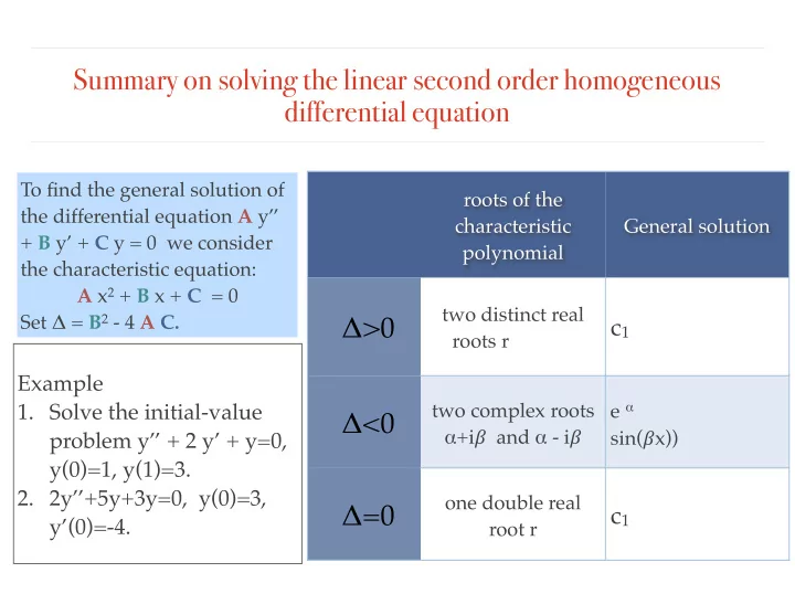
To find the general solution of the differential equation A y’’ + B y’ + C y = 0 we consider the characteristic equation: A x2 + B x + C = 0 Set Δ = B2 - 4 A C. roots of the characteristic polynomial General solution

Δ>0

two distinct real roots r

c1

Δ<0

two complex roots α+i𝛾 and α - i𝛾 e α sin(𝛾x))

Δ=0

• ne double real

root r

c1

Example

• 1. Solve the initial-value

problem y’’ + 2 y’ + y=0, y(0)=1, y(1)=3.

• 2. 2y’’+5y+3y=0, y(0)=3,

y’(0)=-4.

The Logistic Equation

An elementary model of population growth

Assumption: The number of individuals in a population grows at a rate proportional to the size of this population.

The direction of each line represents the slope of the tangent line of the solution passing through the point (t, P(t))

dP/dt = k P k=0.5

M and k are parameters which depend on the population.

k=0.5 and M=100

Another model of population growth

Assumption: The number of individuals in a population grows at a rate proportional to the size

• f this population when the

number of individuals is small, but decreases when surpasses a certain number.

Logistic differential equation dP/dt = k P(1-P/M)

M is the carrying capacity, the amount that when exceeded will result in the population decreasing.

There are two constant solutions of this equations, P(t)=0 and P(t)=M

The direction field of the logistic differential equation and some

• solutions. (M=100, k=0.5)

What are the initial conditions of the plotted solutions?

t = time P (or P(t)) = the population size at time t.

• 1. Solve the initial value problem for logistic

differential equation with initial condition P(0)=P0.

• 2. Study what happens with each solution when

time goes to infinity.

Logistic differential equation dP/dt = k P(1-P/M)

Eleven grizzly bears were introduced to a national park a few years ago. The relative growth rate for grizzly bears is 0.1 and the park can support a maximum of 99 bears. (This is not a realistic relative growth) 1.Assuming a logistic growth model, will the bear population reach 5? 70? 100? 120? 99? 2.Use Euler’s method with step size 2 to estimate the number of bears after 4 years. 3.Use Euler’s method with step size 2 to estimate the number of bears after 4 years assuming the initial number of bears is 44. 4.Find an explicit solution of the corresponding differential equation and check the accuracy of your estimations in 2..

y’(t) = -21 y(t) + e-t y(0) = 0

Example from http://www.ece.uwaterloo.ca/~ece104/

Euler’s method

Suppose a species of fish in lake is modeled by a logistic population model with relative growth rate of k = 0.02 per year and carrying capacity

• f K = 50.

a.Write the differential equation describing the logistic population model for this problem. b.Draw a vector field for this problem. c.Determine the equilibrium solutions for this model. d.If 25 fishes are introduced in the lake, estimate the time it will take to have 8000 fish in the lake.