Structured PVA Historical essay: for example history of protection - PDF document

Final Essay: possible topics Structured PVA Historical essay: for example history of protection of Everglades Concern: Run-off of oil-products from streets/roads Management plan: how to manage the Wakulla river Protection of an endangered species Each essay needs at least 5 citations from the peer-reviewed literature (no websites!). The essay will use these citations to show facts, etc. In the reference list, these 5 used papers need to have a short summary of the paper (about half a page). Example titles from last Vital rates semester (Processes that contribute to change in population size) Coral reef resilience and susceptibility due to human interference Birth and death rates The ripple effect: the consequences of biological control Growth rate Overfishing: without immediate reform the problems of yesterday will be here to stay Fecundity Grizzly bear population management and Grizzly bear-human conflict Conservation efforts towards proper medical waste disposal Vital rates often depend on age and size Endangered species protection and HIV research Each essay needs at least 5 citations from the peer-reviewed literature (no websites!). The essay will use these citations to show facts, etc. In the reference list, these 5 used papers need to have a short summary of the paper (about half a page). 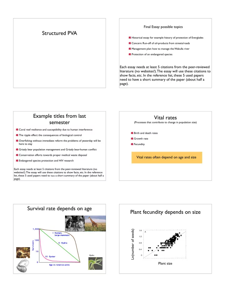Survival rate depends on age Plant fecundity depends on size Ln(number of seeds) Hydra Plant size

Structured (demographic) Types of PVA’s models Age-structured - use data on each age group Count based: simple -- all individuals are the same (age, size, etc.) Structured (demographic): different vital rates for different classes of individuals Structured (demographic) models Building a stage structured model Age-structured - use data on each age group Stage structured - used data on size or stage groups Understand your species Adults > 40 cm Decide how many stages to include Juveniles 20 < x < 40 cm Tadpoles < 20 cm 0 25 50 75 100 0 12.5 25.0 37.5 50.0 Individuals Individuals Building a stage structured model Building a stage structured model (for loggerhead sea turtles) (for loggerhead sea turtles)

How many stages to include? mating near shore foraging Biological Intuition - stages should differ in vital rates from other stages What the data will allow - balance accuracy of more stages open ocean with amount of available data nesting on beaches Life-cycle diagram For turtle PVA we use 5 stages Hatchlings (and eggs): first year Small juveniles: 1-7 years Small Large juveniles: 8-15 years juveniles Subadults 16-21 years (mostly non-breeding) Mature adults 22-55 years, breeding Nestlings Life-cycle diagram Life-cycle diagram Transition rate Stage Large Large juveniles juveniles Small Small Subadults Subadults juveniles juveniles Nestlings Adults Nestlings Adults

Building a stage structured model Understand your species Decide how many stages to include Gather data Turtle data Small Large Mature Nestlings Subadults juveniles juveniles adults Marked in year 1 1000 1000 1000 1000 1000 Recaptured in 0 703 657 682 809 same class Recaptured in 675 47 19 61 - next larger class Eggs/female/year 0 0 0 4.665 61.896 Building a stage structured Life-cycle diagram model Understand your species Large juveniles Decide how many stages to include Gather data Small Calculate transition rates Subadults juveniles Fractions surviving but not growing Fractions surviving and growing Number of female offspring per year and female Nestlings Adults

Life-cycle diagram Turtle data Small Large Mature Nestlings Subadults juveniles juveniles adults Large Marked in year 1 1000 1000 1000 1000 1000 juveniles Recaptured in 0 703 657 682 809 same class Small Subadults juveniles Recaptured in 675 47 19 61 - next larger class 0.675 Eggs/female/year 0 0 0 4.665 61.896 Nestlings Adults Life-cycle diagram Turtle data Small Large Mature Nestlings Subadults juveniles juveniles adults Large Marked in year 1 1000 1000 1000 1000 1000 juveniles Recaptured in 0 703 657 682 809 same class Small Subadults juveniles Recaptured in 675 47 19 61 - next larger class 0.675 Eggs/female/year 0 0 0 4.665 61.896 Nestlings Adults Life-cycle diagram Life-cycle diagram 0.657 0.703 0.703 0.682 Large Large juveniles juveniles 0.047 0.019 Small Small Subadults Subadults juveniles juveniles 4.665 0.061 0.675 Nestlings Adults Nestlings Adults 0.809 61.896 0.703

Building a stage structured Population (Projection) matrix model Understand your species The projection matrix is the Decide how many stages to include summary of all transition probabilities (all vital rates) Gather data Calculate transition rates Make model A generic projection matrix Population (Projection) matrix Size this year 1 2 3 4 5 Number of new turtles (size class 1) produces by F i 1   an average individual of size i per year S 1 F 2 F 3 F 4 F 5 Size 2 G 1 S 2 0 0 0   next   3 0 G 2 S 3 0 0 Fraction of size i turtles surviving and STAYING in S i   year the same size class per year 4   G 3 S 4 0 0 0   5 0 0 0 G 4 S 5 Fraction of size i turtles surviving and GROWING G i to size class i+1 per year F i new S i surviving G i advancing Projection matrix for loggerhead sea turtles Population (Projection) matrix Size this year 1 2 3 4 5 Number of new turtles (size class 1) produces by F i an average individual of size i per year 1   0 0 0 4 . 665 61 . 896 Size 2 0 . 675 0 . 703 0 0 0   next   Fraction of size i turtles surviving and STAYING in S i 3 0 0 . 047 0 . 657 0 0   year the same size class per year   4 0 0 0 . 019 0 . 682 0   5 0 0 0 0 . 061 0 . 8091 Fraction of size i turtles surviving and GROWING G i to size class i+1 per year Note that since S and G are fractions surviving. They are between 0 and 1.

Life-cycle diagram recall count based method 0.657 0.703 0.682 Large N t = λ N t − 1 juveniles 0.047 0.019 Small Subadults juveniles 4.665 0.061 0.675 Nestlings Adults 0.809 61.896 0.703 Structured model Stage distribution vector a column showing the number (or density) of individuals in each stage N t = PN t − 1   Nestlings 23 . 85 Small juveniles 64 . 78     Large juveniles 10 . 33     Subadults 0 . 73   Adults 0 . 31 100.00 Total density Stable stage (or age or size) Stable stage (or age or size) distribution distribution distribution of individuals among stages distribution of individuals among stages that won’t change over time that won’t change over time (if population size changes at a constant rate) (if population size changes at a constant rate) Example: 100% of individuals in Example: 100% of individuals in stage 1 is not stable – the next stage 1 is not stable – the next year there will be individuals in year there will be individuals in other stages other stages Stage distribution will converge to the stable stage distribution over time

N t − 1 N t P       0 0 0 4 . 665 61 . 896 23 . 85 0 . 675 0 . 703 0 0 0 64 . 78       N t = PN t − 1       ? = 0 0 . 047 0 . 657 0 0 10 . 33             0 0 0 . 019 0 . 682 0 0 . 73       0 0 0 0 . 061 0 . 8091 0 . 31 Use matrix algebra..... Eggs N t − 1 N t P Juveniles # Large juveniles Subadults       22 . 59 0 0 0 4 . 665 61 . 896 23 . 85 Adults 61 . 64 0 . 675 0 . 703 0 0 0 64 . 78             9 . 83 = 0 0 . 047 0 . 657 0 0 10 . 33             0 . 69 0 0 0 . 019 0 . 682 0 0 . 73       0 . 30 0 0 0 0 . 061 0 . 8091 0 . 31 Time Same graph as last Eggs Stable stage distribution Juveniles slide, but changing Eggs scale on y-axis Large juveniles # Juveniles Subadults Freq Large juveniles Adults Subadults Adults Time Time

N t − 1 N t P Recall that:       22 . 59 0 0 0 4 . 665 61 . 896 23 . 85 61 . 64 0 . 675 0 . 703 0 0 0 64 . 78       N t       9 . 83 = 0 0 . 047 0 . 657 0 0 10 . 33       λ =       0 . 69 0 0 0 . 019 0 . 682 0 0 . 73       N t − 1 0 . 30 0 0 0 0 . 061 0 . 8091 0 . 31 How do we know if population is growing or shrinking? N t − 1 N t P lambda       22 . 59 0 0 0 4 . 665 61 . 896 23 . 85 61 . 64 0 . 675 0 . 703 0 0 0 64 . 78             9 . 83 = 0 0 . 047 0 . 657 0 0 10 . 33             0 . 69 0 0 0 . 019 0 . 682 0 0 . 73       0 . 30 0 0 0 0 . 061 0 . 8091 0 . 31 95.05 100.0 95.05/100 = 0.9505 = � Time � again � again In a count based model In a count based model N t = λ N t − 1 N t = λ N t − 1 In a structured model In a structured model N t = PN t − 1 N t = PN t − 1 P is playing the same role as the count based � . P is playing the same role as the count based � . The information in P can be summarized by a matrix � (dominant eigenvalue)