SLIDE 18 Applications 3 – C. elegans
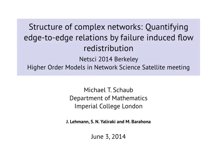
(a)
Head (H) Mid-Body (B) Tail (T)
(b) (c)
Neurons Neurons Sensory Interneurons Motor Neurons Neurons
(d)
IL2VL IL2L IL1VL URADL IL1DL OLLL IL1L URYDL OLQDL URYVL RIPL OLLR IL2R URBL IL1DR URYDR URADR IL1R URAVL OLQVL RMED URBR OLQDR RIPR IL2VR RMEL CEPVL BAGR BAGL OLQVR URAVR RMER IL1VR URYVR CEPVR RMEV CEPDL RMDVL SAAVL SMDVL URXL RID ALA RMDVR CEPDR AVAL RIAL SAAVR RMDL URXR SMDVR AVAR RIAR ASKR ASKL AVEL ADLL ADFL RMDR AFDL AFDR SIBDL RIH AWBL AVER RMDDL AWCL ADFR ASGL SAADL ADLR AWAL AWBR ASIL ASHL SIBDR ASGR AIBL ASHR AWCR AWAR SIBVL RIVL SMDDL SAADR RMHL RMDDR ASIR AVHL AVHR RIVR AIBR RIBL RMFL AVBL SIBVR ASEL AVJ R AUAL SIADL RMHR AVJ L ASER AVBR RIBR RMFR SMDDR AIAL RIR SMBDL RIML ASJ L RIMR AUAR AVDR SMBVR AVDL AINL SMBVL ASJ R AINR SIADR AVL RICL AIAR SMBDR AIZR SIAVL SIAVR RICR AIZL AIYR AIMR AIML RIS AIYL VB02 AVKR AVKL AVFR SABVL FLPL FLPR SABVR AVFL AQR RIFR ADEL VB01 ADER DB02 ADAR ADAL RIGR RMGL RMGR RIFL AVG VA01 SABD RIGL DD01 DB01 AS01 VD01 DA01 VD02 VA02 VB03 AS02 DB03 DA02 VD03 BDUR BDUL VA03 SDQR VB04 VC01 DD02 AS03 VD04 DA03 VA04 VB05 VC02 DB04 AS04 VD05 VA05 AVM VB06 DA04 DD03 ALML ALMR VC03 AS05 VD06 VA06 VB07 DB05 AS06 VD07 VC04 DA05 VC05 HSNR HSNL VA07 VB08 AS07 DD04 VD08 VA08 VB09 DB06 AS08 PDEL VD09 PDER SDQL DA06 PVDL PVM VA09 VB10 AS09 DD05 VD10 VA10 VB1 1 DB07 AS10 DA07 VD1 1 VA1 1 AS1 1 VD12 PVPR PVT VA12 PVPL DA08 DA09 PDB VD13 PDA DVB DVA DVC PVQR PHAL PHAR PVQL LUAL PVCL PHBR ALNL PHBL LUAR ALNR PVCR PQR PVR PVWL PVWR PLNL PHCR PHCL PVNR PLMR PVNL PLML
processing depth normalized Fiedler vector Embeddedness
0.3 0.4 0.5 0.6 0.7 0.8 0.9 sensory neuron interneuron motor neuron