Strategies and Nash Equilibrium A strategy is a specification for how - - PowerPoint PPT Presentation

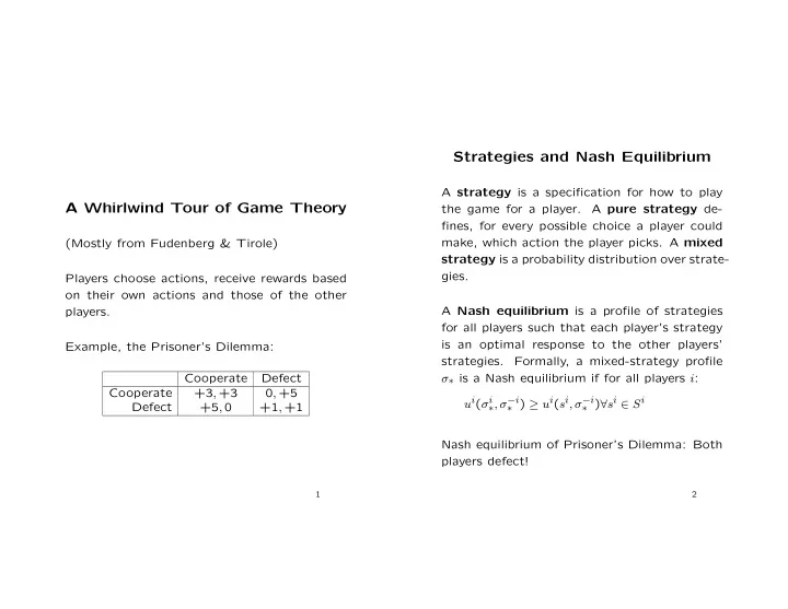
A Whirlwind Tour of Game Theory

(Mostly from Fudenberg & Tirole) Players choose actions, receive rewards based

• n their own actions and those of the other

players. Example, the Prisoner’s Dilemma: Cooperate Defect Cooperate +3, +3 0, +5 Defect +5, 0 +1, +1

1

Strategies and Nash Equilibrium

A strategy is a specification for how to play the game for a player. A pure strategy de- fines, for every possible choice a player could make, which action the player picks. A mixed strategy is a probability distribution over strate- gies. A Nash equilibrium is a profile of strategies for all players such that each player’s strategy is an optimal response to the other players’ strategies. Formally, a mixed-strategy profile σ∗ is a Nash equilibrium if for all players i: ui(σi

∗, σ−i ∗ ) ≥ ui(si, σ−i ∗ )∀si ∈ Si

Nash equilibrium of Prisoner’s Dilemma: Both players defect!

2

Matching Pennies

H T H +1, −1 −1, +1 T −1, +1 +1, −1 No pure strategy equilibria Nash equilibrium: Both players randomize half and half between actions.

3

More on Equilibria

Dominated strategies: Strategy si (strictly) dom- inates strategy s

′

i if, for all possible strategy

combinations of opponents, si yields a (strictly) higher payoff than s

′

i to player i.

Iterated elimination of strictly dominated strate- gies: Eliminate all strategies which are domi- nated, relative to opponents’ strategies which have not yet been eliminated. If iterated elimination of strictly dominated strate- gies yields a unique strategy n-tuple, then this strategy n-tuple is the unique Nash equilibrium (and it is strict). Every Nash equilibrium survives iterated elimi- nation of strictly dominated strategies.

4

Multiple Equilibria

A coordination game: L R U 9, 9 0, 8 D 8, 0 7, 7 U, L and D, R are both Nash equilibria. What would be reasonable to play? With and with-

• ut coordination?

While U, L is pareto-dominant, playing D and R are “safer” for the row and column players respectively...

5

Existence of Equilibria

Nash’s theorem, translated: every game with a finite number of actions for each player where each player’s utilities are consistent with the (previously discussed) axioms of utility theory has an equilibrium in mixed strategies. Idea 1: Reaction correspondences. Player i’s reaction correspondence ri maps each strategy profile σ to the set of mixed strategies that maximize player i’s payoff when her opponents play σ−i. Note that ri depends only on σ−i, so we don’t really need all of σ, but it will be useful to think of it this way. Let r be the Cartesian product of all ri. A fixed point of r is a σ such that σ ∈ r(σ), so that for each player, σi ∈ ri(σ). Thus a fixed point of r is a Nash equilibrium. Kakutani’s FP theorem says that the following are sufficient conditions for r : Σ → Σ to have a FP.

6

• 1. Σ is a compact, convex, nonempty subset
• f a finite-dimensional Euclidean space.

Satisfied, because it’s a simplex

• 2. r(σ) is nonempty for all σ

Each player’s playoffs are linear, and there- fore continuous, in her own mixed strategy. Continuous functions on compact sets at- tain maxima.

• 3. r(σ) is convex for all σ

Suppose not. Then ∃σ

′, σ ′′ such that λσ ′ +

(1 − λ)σ

′′ /

∈ r(σ) But for each player i, ui(λσ

′

i + (1 − λ)σ

′′

i , σ−i) =

λui(σ

′

i, σ−i) + (1 − λ)ui(σ

′′

i , σ−i)

so that if both σ

′ and σ ′′ are best responses

to σ−i, then so is their weighted average.

• 4. r(·) has a closed graph

The correspondence r(·) has a closed graph if the graph of r(·) is a closed set. When- ever the sequence (σn, ˆ σn) → (σ, ˆ σ), with ˆ σn ∈ r(σn)∀n, then ˆ σ ∈ r(σ) (same as up- per hemicontinuity) Suppose that there is a sequence (σn, ˆ σn) → (σ, ˆ σ) such that ˆ σn ∈ r(σn)for every n, but ˆ σ / ∈ r(σ). Then there exists ǫ > 0 and σ′ such that ui(σ

′

i, σ−i) > ui( ˆ

σi, σ−i) + 3ǫ Then, for sufficiently large n, ui(σ

′

i, σn −i) > ui(σ

′

i, σ−i)−ǫ > ui( ˆ

σi, σ−i)+2ǫ > ui(ˆ σn

i , σn −i) + ǫ

which means that σ

′

i does strictly better

against σn

−i than ˆ

σn

i does, contradicting our

assumption.

Learning in Games∗

How do players reach equilibria? What if I don’t know what payoffs my oppo- nent will receive? I can try to learn her actions when we play repeatedly (consider 2-player games for sim- plicity). Fictitious play in two player games. Assumes stationarity of opponent’s strategy, and that players do not attempt to influence each oth- ers’ future play. Learn weight functions κi

t(s−i) = κi t−1(s−i) +

• 1

if s−i

t−1 = s−i

• therwise

∗Fudenberg & Levine,

The Theory of Learning in Games, 1998

7

Calculate probabilities of the other player play- ing various moves as: γi

t(s−i) =

κi

t(s−i)

• ˜

s−i∈S−i κi t(˜

s−i) Then choose the best response action.

Fictitious Play (contd.)

If fictitious play converges, it converges to a Nash equilibrium. If the two players ever play a (strict) NE at time t, they will play it thereafter. (Proofs

• mitted)

If empirical marginal distributions converge, they converge to NE. But this doesn’t mean that play is similar!

t Player1 Action Player2 Action κ1

T

κ2

T

1 T T (1.5, 3) (2, 2.5) 2 T H (2.5, 3) (2, 3.5) 3 T H (3.5, 3) (2, 4.5) 4 H H (4.5, 3) (3, 4.5) 5 H H (5.5, 3) (4, 4.5) 6 H H (6.5, 3) (5, 4.5) 7 H T (6.5, 4) (6, 4.5) Cycling of actions in fictitious play in the matching pennies game

8

Universal Consistency

Persistent miscoordination: Players start with weights of (1, √ 2) A B A 0, 0 1, 1 B 1, 1 0, 0 A rule ρi is said to be ǫ-universally consistent if for any ρ−i lim

T→∞ sup max σi

ui(σi, γi

t)− 1

T

• t

ui(ρi

t(ht−1)) ≤ ǫ

almost surely under the distribution generated by (ρi, ρ−i), where ht−1 is the history up to time t − 1, available for the decision-making algorithm at time t.

9

Back to Experts

Bayesian learning cannot give good payoff guar- antees.

• Suppose the true way your opponent’s ac-

tions are being generated is not in the sup- port of the prior – want protection from unanticipated play, which can be endoge- nously determined.

• The Bayesian optimal method guarantees

a measure of learning something close to the true model, but provides no guarantees

• n received utility.
• Can use the notion of experts to bound

regret!

10

Define universal expertise analogously to uni- versal consistency, and bound regret (lost util- ity) with respect to the best expert, which is a strategy. The best response function is derived by solv- ing the optimization problem max

Ii

Ii ui

t + λvi(Ii)

• ui

t is the vector of average payoffs player i

would receive by using each of the experts Ii is a probability distribution over experts λ is a small positive number. Under technical conditions on v, satisfied by the entropy: −

• s

σ(s) log σ(s) we retrieve the exponential weighting scheme, and for every ǫ there is a λ such that our pro- cedure is ǫ-universally expert.