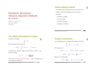
Stochastic Simulation Variance reduction methods Bo Friis Nielsen - PowerPoint PPT Presentation

Stochastic Simulation Variance reduction methods Bo Friis Nielsen Applied Mathematics and Computer Science Technical University of Denmark 2800 Kgs. Lyngby – Denmark Email: bfni@dtu.dk

Variance reduction methods Variance reduction methods • To obtain better estimates (tigher confidence intervals) with the same ressources • Exploit analytical knowledge and/or correlation • Methods: ⋄ Antithetic variables ⋄ Control variates ⋄ Stratified sampling ⋄ Importance sampling ⋄ Common random numbers DTU 02443 – lecture 7 2

Case: Monte Carlo evaluation of integral Case: Monte Carlo evaluation of integral Consider the integral � 1 e x dx 0 We can interpret this interval as � 1 e U � e x dx = θ � E = U ∈ U (0 , 1) 0 To estimate the integral: sample of the random variable e U and take the average. � n i =1 X i ¯ X i = e U i X = n This is the crude Monte Carlo estimator, “crude” because we use no refinements whatsoever. DTU 02443 – lecture 7 3

Analytical considerations Analytical considerations It is straightforward to calculate the integral in this case � 1 e x dx = e − 1 ≈ 1 . 72 0 The estimator X Var ( X ) = E ( X 2 ) − E ( X ) 2 E ( X ) = e − 1 � 1 ( e x ) 2 dx = 1 e 2 − 1 E ( X 2 ) = � � 2 0 Based on one observation Var ( X ) = 1 − ( e − 1) 2 = 0 . 2420 e 2 − 1 � � 2 DTU 02443 – lecture 7 4

Antithetic variables Antithetic variables General idea: to exploit correlation • If the estimator is positively correlated with U i (monotone function): Use 1 − U also = e U i + Y i = e U i + e 1 − U i e � n i =0 Y i e Ui ¯ Y = 2 2 n • The computational effort of calculating ¯ Y should be similar to the effort needed to compute ¯ X . ⋄ By the latter expression of Y i we can generate the same number of Y ’s as X ’s DTU 02443 – lecture 7 5

Antithetic variables - analytical Antithetic variables - analytical We can analyse the example analytically due to its simplicity E ( ¯ Y ) = E ( ¯ X ) = θ To calculate Var ( ¯ Y ) we start with Var ( Y i ) . Var ( Y i ) = 1 + 1 + 2 · 1 e 1 − U i � e U i , e 1 − U i � e U i � � � � 4 Var 4 Var 4 Cov = 1 + 1 e U i � e U i ( e 1 − U i � � � 2 Var 2 Cov e U i , e 1 − U i � e U i e 1 − U i � e 1 − U i � e U i � � � � � Cov = E − E E = e − ( e − 1) 2 = 3 e − e 2 − 1 = − 0 . 2342 Var ( Y i ) = 1 2(0 . 2420 − 0 . 2342) = 0 . 0039 DTU 02443 – lecture 7 6

Comparison: Crude method vs. antithetic Comparison: Crude method vs. antithetic Crude method: Var ( X i ) = 1 − ( e − 1) 2 = 0 . 2420 e 2 − 1 � � 2 Antithetic method: Var ( Y i ) = 1 2(0 . 2420 − 0 . 2342) = 0 . 0039 I.e, a reduction by 98 % , almost for free. The variance on ¯ X - and ¯ Y - will scale with 1 /n , the number of samples. Going from crude to antithetic method, reduces the variance as much as increasing number of samples with a factor 50. DTU 02443 – lecture 7 7

Antethetic variables in more complex models Antethetic variables in more complex models If X = h ( U 1 , . . . , U n ) where h is monotone in each of its coordinates, then we can use antithetic variables Y = h (1 − U 1 , . . . , 1 − U n ) to reduce the variance, because Cov ( X, Y ) ≤ 0 and therefore Var ( 1 2 ( X + Y )) ≤ 1 2 Var ( X ) . DTU 02443 – lecture 7 8

Antithetic variables in the queue simulation Antithetic variables in the queue simulation Can you device the queueing model of yesterday, so that the number of rejections is a monotone function of the underlying U i ’s? Yes: Make sure that we always use either U i or 1 − U i , so that a large U i implies customers arriving quickly and remaining long. DTU 02443 – lecture 7 9

Control variates Control variates Use of covariates Z = X + c ( Y − µ y ) E ( Y ) = µ y ( known ) Var ( Z ) = Var ( X ) + c 2 Var ( Y ) + 2 c Cov ( Y, X ) We can minimize Var ( Z ) by choosing c = − Cov ( X, Y ) Var ( Y ) to get Var ( Z ) = Var ( X ) − Cov ( X, Y ) 2 Var ( Y ) DTU 02443 – lecture 7 10

Example Example Use U as control variate � � U i − 1 X i = e U i Z i = X i + c 2 The optimal value can be found by U, e U � Ue U � e U � � � � Cov ( X, Y ) = Cov = E − E ( U ) E ≈ 0 . 14086 In practice we would not know this covariance, but estimate it empirically. � 2 � e U , U − Cov e U � � Var ( Z c = − 0 . 14086 1 / 12 ) = Var = 0 . 0039 Var ( U ) DTU 02443 – lecture 7 11

Stratified sampling Stratified sampling This is a general survey technique: We sample in predetermined areas, using knowledge of structure of the sampling space Ui, 1 Ui, 2 Ui, 10 1 9 10 + e 10 + 10 + · · · + e 10 + W i = e 10 10 What is an appropriate number of strata? (In this case there is a simple answer; for complex problems not so) DTU 02443 – lecture 7 12

Importance sampling Importance sampling Suppose we want to evaluate � θ = E ( h ( X )) = h ( x ) f ( x ) dx For g ( x ) > 0 whenever f ( x ) > 0 this is equivalent to � h ( x ) f ( x ) � h ( Y ) f ( Y ) � θ = g ( x ) dx = E g ( x ) g ( Y ) where Y is distributed with density g ( y ) This is an efficient estimator of θ , if we have chosen g such that the � � h ( Y ) f ( Y ) variance of is small. g ( Y ) Such a g will lead to more Y ’s where h ( y ) is large. More important regions will be sampled more often. DTU 02443 – lecture 7 13

Re-using the random numbers Re-using the random numbers We want to compare two different queueing systems. We can estimate the rejection rate of system i = 1 , 2 by θ i = E ( g i ( U 1 , . . . , U n )) and then rate the two systems according to θ 2 − ˆ ˆ θ 1 But typically g 1 ( · · · ) and g 2 ( · · · ) are positively correlated: Long service times imply many rejections. DTU 02443 – lecture 7 14

Then a more efficient estimator is based on θ 2 − θ 1 = E ( g 2 ( U 1 , . . . , U n ) − g 1 ( U 1 , . . . , U n )) This amounts to letting the two systems run with the same input sequence of random numbers, i.e. same arrival and service time for each customer. With some program flows, this is easily obtained by re-setting the seed of the RNG. When this is not sufficient, you must store the sequence of arrival and service times, so they can be re-used. Note: In the slides there is no gain, as we make only one run! DTU 02443 – lecture 7 15

Exercise 5: Variance reduction methods Exercise 5: Variance reduction methods � 1 0 e x dx by simulation (the crude Monte Carlo 1. Estimate the integral estimator). Use eg. an estimator based on 100 samples and present the result as the point estimator and a confidence interval. � 1 0 e x dx using antithetic variables, with 2. Estimate the integral comparable computer ressources. � 1 0 e x dx using a control variable, with 3. Estimate the integral comparable computer ressources. � 1 0 e x dx using stratified sampling, with 4. Estimate the integral comparable computer ressources. 5. Use control variates to reduce the variance of the estimator in exercise 4 (Poisson arrivals). 6. Demonstrate the effect of using common random numbers in exercise 4 for the difference between Poisson arrivals (Part 1) and a renewal process with hyperexponential interarrival times. Remark: You might need to some thinking and some re-programming.