Stochastic Simulation Methods: Variance reduction methods - PowerPoint PPT Presentation

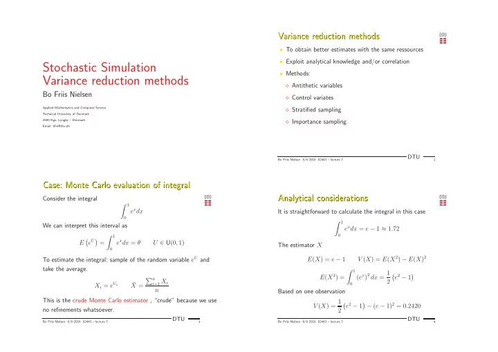
Variance reduction methods Variance reduction methods • To obtain better estimates with the same ressources • Exploit analytical knowledge and/or correlation Stochastic Simulation • Methods: Variance reduction methods ⋄ Antithetic variables Bo Friis Nielsen ⋄ Control variates Applied Mathematics and Computer Science ⋄ Stratified sampling Technical University of Denmark 2800 Kgs. Lyngby – Denmark ⋄ Importance sampling Email: bfni@dtu.dk DTU Bo Friis Nielsen 8/6 2016 02443 – lecture 7 2 Case: Monte Carlo evaluation of integral Case: Monte Carlo evaluation of integral Analytical considerations Analytical considerations Consider the integral � 1 e x dx It is straightforward to calculate the integral in this case 0 � 1 We can interpret this interval as e x dx = e − 1 ≈ 1 . 72 � 1 0 e U � e x dx = θ � E = U ∈ U (0 , 1) The estimator X 0 To estimate the integral: sample of the random variable e U and V ( X ) = E ( X 2 ) − E ( X ) 2 E ( X ) = e − 1 take the average. � 1 ( e x ) 2 dx = 1 e 2 − 1 E ( X 2 ) = � � � n i =1 X i 2 ¯ X i = e U i 0 X = n Based on one observation This is the crude Monte Carlo estimator , “crude” because we use V ( X ) = 1 − ( e − 1) 2 = 0 . 2420 e 2 − 1 � � no refinements whatsoever. 2 DTU DTU Bo Friis Nielsen 8/6 2016 02443 – lecture 7 3 Bo Friis Nielsen 8/6 2016 02443 – lecture 7 4

Antithetic variables - analytical Antithetic variables - analytical Antithetic variables Antithetic variables We can analyse the example analytically due to its simplicity General idea: to exploit correlation E ( ¯ Y ) = E ( ¯ X ) = θ • If the estimator is positively correlated with U i (monotone function): Use 1 − U also To calculate V ( ¯ Y ) we start with V ( Y i ) . = e U i + Y i = e U i + e 1 − U i e � n i =0 Y i V ( Y i ) = 1 + 1 + 2 · 1 e Ui ¯ Y = � e U i � � e 1 − U i � � e U i , e 1 − U i � 4 V 4 V 4 Cov 2 2 n = 1 + 1 • The computational effort of calculating ¯ Y should be similar to e U i � e U i ( e 1 − U i � � � 2 V 2 Cov the effort needed to compute ¯ X . e U i , e 1 − U i � e U i e 1 − U i � e 1 − U i � � � � e U i � � Cov = E − E E ⋄ By the latter expression of Y i we can generate the same = e − ( e − 1) 2 = 3 e − e 2 − 1 = − 0 . 2342 number of Y ’s as X ’s V ( Y i ) = 1 2(0 . 2420 − 0 . 2342) = 0 . 0039 DTU DTU Bo Friis Nielsen 8/6 2016 02443 – lecture 7 5 Bo Friis Nielsen 8/6 2016 02443 – lecture 7 6 Comparison: Crude method vs. antithetic Comparison: Crude method vs. antithetic Antethetic variables in more complex models Antethetic variables in more complex models Crude method: If X = h ( U 1 , . . . , U n ) V ( X i ) = 1 − ( e − 1) 2 = 0 . 2420 e 2 − 1 � � 2 where h is monotone in each of its coordinates, then we can use Antithetic method: antithetic variables V ( Y i ) = 1 2(0 . 2420 − 0 . 2342) = 0 . 0039 Y = h (1 − U 1 , . . . , 1 − U n ) I.e, a reduction by 98 % , almost for free. to reduce the variance, because The variance on ¯ X - and ¯ Y - will scale with 1 /n , the number of Cov( X, Y ) ≤ 0 samples. and therefore V ( 1 2 ( X + Y )) ≤ 1 2 V X . Going from crude to antithetic method, reduces the variance as much as increasing number of samples with a factor 50. DTU DTU Bo Friis Nielsen 8/6 2016 02443 – lecture 7 7 Bo Friis Nielsen 8/6 2016 02443 – lecture 7 8

Antithetic variables in the queue simulation Antithetic variables in the queue simulation Control variates Control variates Can you device the queueing model of yesterday, so that the Use of covariates number of rejections is a monotone function of the underlying U i ’s? Z = X + c ( Y − µ y ) E ( Y ) = µ y ( known ) V ( Z ) = V ( X ) + c 2 V ( Y ) + 2 cCov ( Y, X ) Yes: Make sure that we always use either U i or 1 − U i , so that a We can minimize V ( Z ) by choosing large U i implies customers arriving quickly and remaining long. c = − Cov ( X, Y ) V ( Y ) to get V ( Z ) = V ( X ) − Cov ( X, Y ) 2 V ( Y ) DTU DTU Bo Friis Nielsen 8/6 2016 02443 – lecture 7 9 Bo Friis Nielsen 8/6 2016 02443 – lecture 7 10 Example Example Stratified sampling Stratified sampling Use U as control variate This is a general survey technique: We sample in predetermined areas, using knowledge of structure of the sampling space � U i − 1 � X i = e U i Z i = X i + c 2 Ui, 1 Ui, 2 Ui, 10 1 9 10 + e 10 + 10 + · · · + e 10 + W i = e The optimal value can be found by 10 10 � U, e U � � Ue U � � e U � Cov ( X, Y ) = Cov = E − E ( U ) E ≈ 0 . 14086 What is an appropriate number of strata? (In this case there is a simple answer; for complex problems not so) In practice we would not know this covariance, but estimate it empirically. � 2 � − Cov e U , U � e U � V ( Z c = − 0 . 14086 1 / 12 ) = V = 0 . 0039 V ( U ) DTU DTU Bo Friis Nielsen 8/6 2016 02443 – lecture 7 11 Bo Friis Nielsen 8/6 2016 02443 – lecture 7 12

Importance sampling Importance sampling Suppose we want to evaluate Re-using the random numbers Re-using the random numbers � We want to compare two different queueing systems. θ = E ( h ( X )) = h ( x ) f ( x ) dx We can estimate the rejection rate of system i = 1 , 2 by For g ( x ) > 0 whenever f ( x ) > 0 this is equivalent to � h ( x ) f ( x ) θ i = E g i ( U 1 , . . . , U n ) � h ( Y ) f ( Y ) � θ = g ( x ) dx = E g ( x ) g ( Y ) and then rate the two systems according to where Y is distributed according to g ( y ) θ 2 − ˆ ˆ θ 1 This is an efficient estimator of θ , if we have chosen g such that the � � h ( Y ) f ( Y ) But typically g 1 ( · · · ) and g 2 ( · · · ) are positively correlated: Long variance of is small. g ( Y ) service times imply many rejections. Such a g will lead to more Y ’s where h ( y ) is large. More important regions will be sampled more often. DTU DTU Bo Friis Nielsen 8/6 2016 02443 – lecture 7 13 Bo Friis Nielsen 8/6 2016 02443 – lecture 7 14 Exercise 5: Variance reduction methods Exercise 5: Variance reduction methods � 1 0 e x dx by simulation (the crude Monte • Estimate the integral Then are more efficient estimator is based on Carlo estimator). Use eg. an estimator based on 100 samples θ 2 − θ 1 = E ( g 2 ( U 1 , . . . , U n ) − g 1 ( U 1 , . . . , U n )) and present the result as the point estimator and a confidence interval. This amounts to letting the two systems run with the same input � 1 • Estimate the integral 0 e x dx using antithetic variables, with sequence of random numbers, i.e. same arrival and service time for comparable computer ressources. each customer. � 1 0 e x dx using a control variable, with • Estimate the integral With some program flows, this is easily obtained by re-setting the comparable computer ressources. seed of the RNG. � 1 0 e x dx using stratified sampling, with • Estimate the integral When this is not sufficient, you must store the sequence of arrival comparable computer ressources. and service times, so they can be re-used. • Optional: Use control variates to reduce the variance of the estimator in exercise 4 (Poisson arrivals). DTU DTU Bo Friis Nielsen 8/6 2016 02443 – lecture 7 15 Bo Friis Nielsen 8/6 2016 02443 – lecture 7 16