steady state simulation
play

Steady-State Simulation Steady-State Simulation Overview Reading: - PowerPoint PPT Presentation

Steady-State Simulation Steady-State Simulation Overview Reading: Ch. 9 in Law & Ch. 15 in Handbook of Simulation The Regenerative Method Regenerative processes Regenerative Simulation Peter J. Haas Delays The Batch Means Method


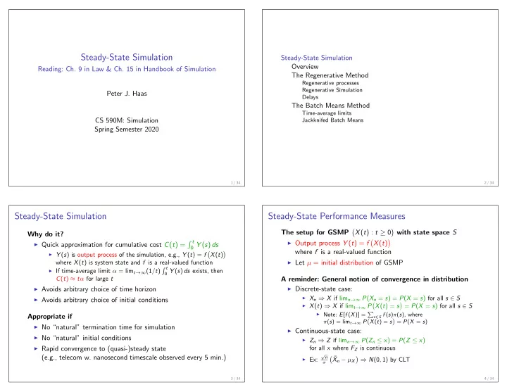
  1. Steady-State Simulation Steady-State Simulation Overview Reading: Ch. 9 in Law & Ch. 15 in Handbook of Simulation The Regenerative Method Regenerative processes Regenerative Simulation Peter J. Haas Delays The Batch Means Method Time-average limits CS 590M: Simulation Jackknifed Batch Means Spring Semester 2020 1 / 34 2 / 34 Steady-State Simulation Steady-State Performance Measures � � The setup for GSMP X ( t ) : t ≥ 0 with state space S Why do it? � t ◮ Output process Y ( t ) = f � � X ( t ) ◮ Quick approximation for cumulative cost C ( t ) = 0 Y ( s ) ds where f is a real-valued function ◮ Y ( s ) is output process of the simulation, e.g., Y ( t ) = f � � X ( t ) ◮ Let µ = initial distribution of GSMP where X ( t ) is system state and f is a real-valued function � t ◮ If time-average limit α = lim t →∞ (1 / t ) 0 Y ( s ) ds exists, then C ( t ) ≈ t α for large t A reminder: General notion of convergence in distribution ◮ Avoids arbitrary choice of time horizon ◮ Discrete-state case: ◮ X n ⇒ X if lim n →∞ P ( X n = s ) = P ( X = s ) for all s ∈ S ◮ Avoids arbitrary choice of initial conditions ◮ X ( t ) ⇒ X if lim t →∞ P � � X ( t ) = s = P ( X = s ) for all s ∈ S ◮ Note: E [ f ( X )] = � s ∈ S f ( s ) π ( s ), where Appropriate if � � π ( s ) = lim t →∞ P X ( t ) = s = P ( X = s ) ◮ No “natural” termination time for simulation ◮ Continuous-state case: ◮ No “natural” initial conditions ◮ Z n ⇒ Z if lim n →∞ P ( Z n ≤ x ) = P ( Z ≤ x ) ◮ Rapid convergence to (quasi-)steady state for all x where F Z is continuous � ¯ √ n (e.g., telecom w. nanosecond timescale observed every 5 min.) ◮ Ex: � X n − µ X ⇒ N (0 , 1) by CLT σ 3 / 34 4 / 34

  2. Steady-State Performance Measures, Continued Steady-State Simulation Challenges Time-Average Limit of Y ( t ) process Autocorrelation problem � t � � ◮ For time-average limit, α such that P µ lim t →∞ (1 / t ) 0 Y ( u ) du = α = 1 for any µ � t α = lim t →∞ ¯ Y ( t ) = lim t →∞ (1 / t ) 0 Y ( u ) du ◮ Natural estimator of α is ¯ Y ( t ) for some large t Steady-State Mean of Y ( t ) process (obtained from one long observation of system) α = E [ f ( X )], where, for any µ , X ( t ) ⇒ X and E [ f ( X )] exists ◮ But Y ( t ) and Y ( t + ∆ t ) highly correlated if ∆ t is small ◮ So estimator is average of autocorrelated observations Limiting Mean of Y ( t ) process ◮ Techniques based on i.i.d. observations don’t work � � �� α = lim t →∞ E f X ( t ) for any µ Initial-Transient Problem ◮ “for any µ ” = for any member of GSMP family indexed by µ ◮ Steady-state distribution unknown, (with other building blocks the same) so initial dist’n is not typical of steady-state behavior ◮ E [ f ( X )] exists if and only if E [ | f ( X ) | ] < ∞ ◮ Autocorrelation implies that initial bias will persist ◮ If f is bounded or S is finite, then X ( t ) ⇒ X implies ◮ Very hard to detect “end of initial-transient period” � � �� lim t →∞ E X ( t ) = E [ f ( X )] (s-s mean = limiting mean) f 5 / 34 6 / 34 Estimation Methods Many alternative estimation methods ◮ Regenerative method Steady-State Simulation ◮ Batch-means method Overview ◮ Autoregressive method The Regenerative Method Regenerative processes ◮ Standardized-time-series methods Regenerative Simulation ◮ Integrated-path method Delays The Batch Means Method ◮ . . . Time-average limits Jackknifed Batch Means We will focus on: ◮ Regenerative method: clean and elegant ◮ Batch means: simple, widely used and the basis for other methods 7 / 34 8 / 34

  3. The Regenerative Method Regenerative Processes: Formal Definition Definition: Stopping time A random variable T is a stopping time with respect to References: � � X ( t ) : t ≥ 0 if occurrence or non-occurrence of event { T ≤ t } is ◮ Shedler [Ch. 2 & 3], Haas [Ch. 5 & 6] � � completely determined by X ( u ) : 0 ≤ u ≤ t ◮ Recent developments: ACM TOMACS 25(4), 2015 Definition: Regenerative process Regenerative Processes � � The process X ( t ) : t ≥ 0 is regenerative if there exists an infinite ◮ Intuitively: � � X ( t ) : t ≥ 0 is regenerative if process � � sequence of a.s. finite stopping times T ( k ) : k ≥ 0 s.t. for k ≥ 1 “probabilistically restarts” infinitely often � X ( t ) : t ≥ T ( k ) � � X ( t ) : t ≥ T (0) � 1. is distributed as ◮ Restart times T (0) , T (1) , . . . called regeneration times or � � � � regeneration points 2. X ( t ) : t ≥ T ( k ) is independent of X ( t ) : t < T ( k ) ◮ Regeneration points are random ◮ Must be almost surely (a.s.) finite ◮ If T (0) = 0, process is non-delayed (else delayed) ◮ Ex: Arrivals to empty GI/G/1 queue ◮ Can drop stopping-time requirement, (more complicated def.) ◮ � � � � � � X ( t ) : t ≥ 0 regen. ⇒ f X ( t ) : t ≥ 0 regen. ◮ Analogous definition for discrete-time processes 9 / 34 10 / 34 Regenerative Processes: Examples Regenerative GSMPs Ex 3: GSMP with a single state ◮ ¯ s ∈ S is a single state if E (¯ s ) = { ¯ e } for some ¯ e ∈ E Ex 1: Successive times that CTMC hits a fixed state x ◮ Regeneration points: successive times that ¯ e occurs in ¯ s ◮ Formally, T (0) = 0 and ◮ Observe that for each k ≥ 1, T ( k ) = min { t > T ( k − 1) : X ( t − ) � = x and X ( t ) = x } ◮ New state s ′ at T ( k ) distributed according to p ( · ; ¯ s , ¯ e ) ◮ Observe that X � � T ( k ) = x for all k ◮ No old clocks ◮ The two regenerative criteria follow from Markov property ◮ Clock for new event e ′ distributed as F ( · ; s ′ , e ′ , ¯ s , ¯ e ) ◮ Regenerative property follows from Markov property for Ex 2: Successive times that CTMC leaves a fixed state x � ( S n , C n ) : n ≥ 0 � ◮ X � � T ( k ) distributed according to P ( x , · ) for each k ◮ Second criterion follows from Markov property Ex 4: GI/G/1 queue ◮ X ( t ) = number of jobs in system at time t Q: Is a semi-Markov process regenerative? ◮ � � X ( t ) : t ≥ 0 is a GSMP ◮ T ( k ) = time of k th arrival to empty system (why?) 11 / 34 12 / 34

  4. Regenerative GSMPs, Continued Ex 5: Cancellation ◮ Suppose there exist ¯ s ′ , ¯ s ∈ S and ¯ e ∈ E (¯ s ) with s ′ ; ¯ s ′ ; ¯ e ) = ∅ p (¯ s , ¯ e ) r (¯ s , ¯ e ) > 0 such that O (¯ s , ¯ Steady-State Simulation ◮ T ( k ) = k th time that ¯ e occurs in ¯ s and new state is ¯ s ′ Overview The Regenerative Method Ex 6: Exponential clocks Regenerative processes Regenerative Simulation ◮ Suppose that Delays ◮ There exists ˜ E ⊆ E such that each e ∈ ˜ E is a simple event The Batch Means Method with F ( x ; e ) = 1 − e − λ ( e ) x Time-average limits e } ⊆ ˜ ◮ There exists ¯ s ∈ S and ¯ e ∈ E (¯ s ) − { ¯ s ) s.t. E (¯ E Jackknifed Batch Means ◮ T ( k ) = k th time that ¯ e occurs in ¯ s (memoryless property) Other (fancier) regeneration point constructions are possible ◮ E.g., if clock-setting distn’s have heavier-than-exponential � � tails or bounded hazard rates h ( t ) = f ( t ) / 1 − F ( t ) 13 / 34 14 / 34 Regenerative Simulation: Cycles Regenerative Simulation: Time-Average Limits � t ◮ Recall: ¯ Y ( t ) = (1 / t ) 0 Y ( u ) du Theorem Suppose that E [ | Y 1 | ] < ∞ and E [ τ 1 ] < ∞ . Then lim t →∞ ¯ Y ( t ) = α a.s., where α = E [ Y ] / E [ τ ]. ◮ So estimating time-average limit reduces to a ratio-estimation Regeneration points decompose process into i.i.d. cycles problem (can use delta method, jackknife, bootstrap) ◮ k th cycle: � X ( t ) : T ( k − 1) ≤ t < T ( k ) � (Most of) Proof ◮ Length of k th cycle: τ k = T ( k ) − T ( k − 1) � T ( k ) ◮ Set Y k = � T ( j ) T ( k − 1) Y ( u ) du � n � T ( n ) � n T ( j − 1) Y ( u ) du j =1 Y j 1 j =1 ¯ � � � = Y T ( n ) = Y ( u ) du = ◮ The pairs ( Y 1 , τ 1 ) , ( Y 2 , τ 2 ) , . . . are i.i.d as ( Y , τ ) � n � n � T ( n ) T ( j ) − T ( j − 1) j =1 τ j 0 j =1 ¯ ⇒ lim � � Y T ( n ) = α a.s. by SLLN Initial transient is not a problem! n →∞ 15 / 34 16 / 34

Download Presentation
Download Policy: The content available on the website is offered to you 'AS IS' for your personal information and use only. It cannot be commercialized, licensed, or distributed on other websites without prior consent from the author. To download a presentation, simply click this link. If you encounter any difficulties during the download process, it's possible that the publisher has removed the file from their server.

Recommend


More recommend