Steady State Equation for Wells After a well has been pumped for - - PowerPoint PPT Presentation

Steady State Equation for Wells

• After a well has been pumped for an extended period, steady state

conditions are approached

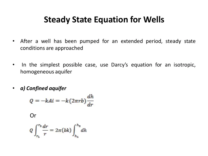
• In the simplest possible case, use Darcy’s equation for an isotropic,

homogeneous aquifer

• a) Confined aquifer

Or

Steady State Equation for Wells (cont.)

• Therefore,

where T is known as the transmissivity and is equal to (bk). The above equation is known as Thiem equation

• Drawdown = H – h =
• Where, R is the radius of influence and rw is the radius of well

• b) Unconfined aquifer

;

• Integrate from r1 to r2.
• If the drawdown is small compared to the thickness of the aquifer, then

(h1 + h2)/2 is approximately equal to H and the equation reduces to steady state confined well equation

Steady State Equation for Wells (cont.)

Well Interference

Assumptions

• In unconfined aquifers, usually two assumptions are involved
• Dupuit’s approximation:

1) The gradient of the piezometric head is constant over any vertical section and is equal to at the free surface. 2) The velocity is horizontal and uniform from top to bottom of any vertical section

Problem

• For the flow through a dike shown in the figure, find the equation of the

free surface. Determine the discharge per unit length of dike in terms of L and the heads at the two boundaries

H H1

L

x

Solution

• r
• At x = L, H = H1
• Therefore,

General Observations

General Observations (cont.)

Groundwater Flow Problem : 1

• An unconfined aquifer is used as a municipal water supply. A railroad car

derailed and contaminated the aquifer 3.0 km up gradient (slope = 0.005). Estimate the travel time for the contaminated groundwater to reach the water supply, if the intrinsic permeability of the aquifer is 100 darcy and the effectiveporosity is 0.15.

• Determine the maximum steady-state pumping rate in lps for a 300-mm

diameter well completed in a confined aquifer with a transmissivity of 124 m2/day. The maximum allowable drawdown at the well is limited to 61.0

• m. The radius of influence for the well is 18,000 m.

Groundwater Flow Problem : 2

• In the sketch below, an unconfined aquifer on a hillside drains into a
• stream. The aquifer has an average saturated thickness of 3.0 m, has a

hydraulic conductivity of 0.30 m/day, an effective porosity of 0.20 and a slope of 0.03. Compute the maximum seepage into the stream per km considering seepage is from both sides of the channel. Compute the travel time for water to flow from the ridge to the channel, 300 m away.

Groundwater Flow Problem : 3