Statistical Learning Learning From Examples We want to estimate - PowerPoint PPT Presentation

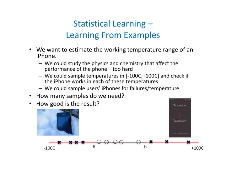
Statistical Learning – Learning From Examples • We want to estimate the working temperature range of an iPhone. – We could study the physics and chemistry that affect the performance of the phone – too hard – We could sample temperatures in [-100C,+100C] and check if the iPhone works in each of these temperatures – We could sample users’ iPhones for failures/temperature • How many samples do we need? • How good is the result? a b -100C +100C

Sample Complexity Sample Complexity answers the fundamental ques7ons in machine learning / sta7s7cal learning / data mining / data analysis: • Does the data (training set) contains sufficient informa7on to make a valid predic7on (or fix a model)? • Is the sample sufficiently large? • How accurate is a predic7on (model) inferred from a sample of a given size? Standard sta7s7cs/probabilis7c techniques do not give adequate solu7ons

Outline • Example: Learning binary classification • Detection vs. estimation • Uniform convergence • VC-dimension • The ε-net and ε-sample theorems • Applications in learning and data analysis • Rademacher complexity • Applications of Rademacher complexity

Example • An alien arrives in Providence. He has a perfect infrared sensors that detects the temperature. He wants to know when the locals say that it’s warm (in contrast to cold or hot) so he can speak like a local. • He asks everyone he meets and gets a collections of answers: (90 F , hot ) , (40 F , cold ) , (60 F , warm ) , (85 F , hot ) , (75 F , warm ) , (30 F , cold ) , (55 F , warm ) .... • He decides that the locals use warm for temperatures between 47.5F to 80F. How wrong can he be? • How do we measure ”wrong”? • How about inconsistent training example? • ...

What’s Learning? Two types of learning: What’s a rectangle? • ”A rectangle is any quadrilateral with four right angles” • Here are many random examples of rectangles, here are many random examples of shapes that are not rectangles. Make your own rule that best conforms with the examples - Statistical Learning.

Learning From Examples • The alien had n random training examples from distribution D . A rule [ a , b ] conforms with the examples. • The alien uses this rule to decide on the next example. • If the next example is drawn from D , what is the probability that he is wrong? • Let [ c , d ] be the correct rule. • Let ∆ = ([ a , b ] − [ c , d ]) ∪ ([ c , d ] − [ a , b ]) • The alien is wrong only on examples in ∆.

What’s the probability that the alien is wrong? • The alien is wrong only on examples in ∆. • The probability that the alien is wrong is the probability of having a quary from ∆. • If Prob (sample from ∆) ≤ ǫ we don’t care. • If Prob (sample from ∆) ≥ ǫ then the probability that n training samples all missed ∆, is bounded by (1 − ǫ ) n = δ , for n ≥ 1 ǫ log 1 δ . • Thus, with n ≥ 1 ǫ log 1 δ training samples, with probability 1 − δ , we chose a rule (interval) that gives the correct answer for quarries from D with probability ≥ 1 − ǫ .

Learning a Binary Classifier • An unknown probability distribution D on a domain U • An unknown correct classification – a partition c of U to In and Out sets • Input: • Concept class C – a collection of possible classification rules (partitions of U ). • A training set { ( x i , c ( x i )) | i = 1 , . . . , m } , where x 1 , . . . , x m are sampled from D . • Goal: With probability 1 − δ the algorithm generates a good classifier. A classifier is good if the probability that it errs on an item generated from D is ≤ opt ( C ) + ǫ , where opt ( C ) is the error probability of the best classifier in C .

Learning a Binary Classifier • Out and In items, and a concept class C of possible classifica;on rules

When does the sample identify the correct rule? - The realizable case • The realizable case - the correct classification c ∈ C . • For any h ∈ C let ∆( c , h ) be the set of items on which the two classifiers differ: ∆( c , h ) = { x ∈ U | h ( x ) � = c ( x ) } • Algorithm: choose h ∗ ∈ C that agrees with all the training set (there must be at least one). • If the sample (training set) intersects every set in { ∆( c , h ) | Pr (∆( c , h )) ≥ ǫ } , then Pr (∆( c , h ∗ )) ≤ ǫ.

Learning a Binary Classifier • Red and blue items, possible classifica9on rules, and the sample items

When does the sample identify the correct rule? The unrealizable (agnostic) case • The unrealizable case - c may not be in C . • For any h ∈ C , let ∆( c , h ) be the set of items on which the two classifiers differ: ∆( c , h ) = { x ∈ U | h ( x ) � = c ( x ) } • For the training set { ( x i , c ( x i )) | i = 1 , . . . , m } , let m Pr (∆( c , h )) = 1 ˜ � 1 h ( x i ) � = c ( x i ) m i =1 • Algorithm: choose h ∗ = arg min h ∈C ˜ Pr (∆( c , h )) . • If for every set ∆( c , h ), | Pr (∆( c , h )) − ˜ Pr (∆( c , h )) | ≤ ǫ, then Pr (∆( c , h ∗ )) ≤ opt ( C ) + 2 ǫ. where opt ( C ) is the error probability of the best classifier in C .

If for every set ∆( c , h ), | Pr (∆( c , h )) − ˜ Pr (∆( c , h )) | ≤ ǫ, then Pr (∆( c , h ∗ )) ≤ opt ( C ) + 2 ǫ. where opt ( C ) is the error probability of the best classifier in C . Let ¯ h be the best classifier in C . Since the algorithm chose h ∗ , Pr (∆( c , h ∗ )) ≤ ˜ ˜ Pr (∆( c , ¯ h )) . Thus, ˜ Pr (∆( c , h ∗ )) − opt ( C ) Pr (∆( c , h ∗ )) − opt ( C ) + ǫ ≤ Pr (∆( c , ¯ ˜ ≤ h )) − opt ( C ) + ǫ ≤ 2 ǫ

Detection vs. Estimation • Input: • Concept class C – a collection of possible classification rules (partitions of U ). • A training set { ( x i , c ( x i )) | i = 1 , . . . , m } , where x 1 , . . . , x m are sampled from D . • For any h ∈ C , let ∆( c , h ) be the set of items on which the two classifiers differ: ∆( c , h ) = { x ∈ U | h ( x ) � = c ( x ) } • For the realizable case we need a training set (sample) that with probability 1 − δ intersects every set in { ∆( c , h ) | Pr (∆( c , h )) ≥ ǫ } ( ǫ -net) • For the unrealizable case we need a training set that with probability 1 − δ estimates, within additive error ǫ , every set in ∆( c , h ) = { x ∈ U | h ( x ) � = c ( x ) } ( ǫ -sample) .

Learnability - Uniform Convergence Theorem In the realizable case, any concept class C can be learned with m = 1 ǫ (ln |C| + ln 1 δ ) samples. Proof. We need a sample that intersects every set in the family of sets { ∆( c , c ′ ) | Pr (∆( c , c ′ )) ≥ ǫ } . There are at most |C| such sets, and the probability that a sample is chosen inside a set is ≥ ǫ . The probability that m random samples did not intersect with at least one of the sets is bounded by |C| (1 − ǫ ) m ≤ |C| e − ǫ m ≤ |C| e − (ln |C| +ln 1 δ ) ≤ δ.

How ¡Good ¡is ¡this ¡Bound? ¡ • Assume ¡that ¡we ¡want ¡to ¡es3mate ¡the ¡working ¡ temperature ¡range ¡of ¡an ¡iPhone. ¡ • We ¡sample ¡temperatures ¡in ¡[-­‑100C,+100C] ¡ and ¡check ¡if ¡the ¡iPhone ¡works ¡in ¡each ¡of ¡these ¡ temperatures. ¡ a ¡ b ¡ -­‑100C ¡ +100C ¡

Learning an Interval • A distribution D is defined on universe that is an interval [ A , B ]. • The true classification rule is defined by a sub-interval [ a , b ] ⊆ [ A , B ]. • The concept class C is the collection of all intervals, C = { [ c , d ] | [ c , d ] ⊆ [ A , B ] } Theorem There is a learning algorithm that given a sample from D of size m = 2 ǫ ln 2 δ , with probability 1 − δ , returns a classification rule (interval) [ x , y ] that is correct with probability 1 − ǫ . Note that the sample size is independent of the size of the concept class |C| , which is infinite.

Learning ¡an ¡Interval ¡ • If ¡the ¡classifica2on ¡error ¡is ¡≥ ¡ε ¡then ¡the ¡sample ¡ missed ¡at ¡least ¡one ¡of ¡the ¡the ¡intervals ¡[a,a’] ¡ or ¡[b’,b] ¡each ¡of ¡probability ¡≥ ¡ε/2 ¡ ¡ ε/2 ¡ ε/2 ¡ a’ ¡ b’ ¡ b ¡ A ¡ a ¡ B ¡ x ¡ y ¡ Each ¡sample ¡excludes ¡many ¡possible ¡intervals. ¡ The ¡union ¡bound ¡sums ¡over ¡overlapping ¡hypothesis. ¡ Need ¡beIer ¡characteriza2on ¡of ¡concept's ¡complexity! ¡ ¡

Proof. Algorithm: Choose the smallest interval [ x , y ] that includes all the ”In” sample points. • Clearly a ≤ x < y ≤ b , and the algorithm can only err in classifying ”In” points as ”Out” points. • Fix a < a ′ and b ′ < b such that Pr ([ a , a ′ ]) = ǫ/ 2 and Pr ([ b , b ′ ]) = ǫ/ 2. • If the probability of error when using the classification [ x , y ] is ≥ ǫ then either a ′ ≤ x or y ≤ b ′ or both. • The probability that the sample of size m = 2 ǫ ln 2 δ did not intersect with one of these intervals is bounded by 2(1 − ǫ 2) m ≤ e − ǫ m 2 +ln 2 ≤ δ

• The union bound is far too loose for our applications. It sums over overlapping hypothesis. • Each sample excludes many possible intervals. • Need better characterization of concept’s complexity!