Statistical Geometry Processing Winter Semester 2011/2012 - PowerPoint PPT Presentation

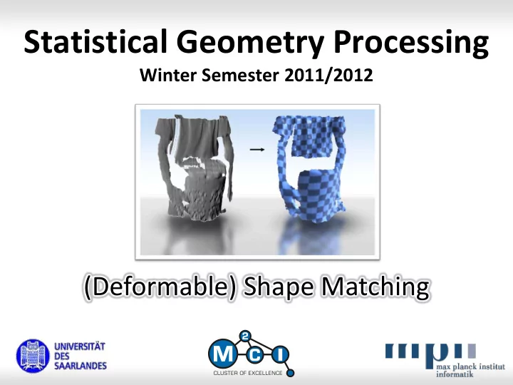
Statistical Geometry Processing Winter Semester 2011/2012 (Deformable) Shape Matching

Rigid Shape Matching

Iterated Closest Points (ICP) Part B (moves, rotation & translation) Part A (stays fixed) The main idea: • Pairwise matching technique  Registers two scans  Multi-part matching is a different story (more on this later) • We want to minimize the distance between the two parts  We set up a variational problem  Minimize distance “energy” by rigid motion of one part 3

Iterated Closest Points (ICP) Problem: • How to compute the distance • This is simple if we know the corresponding points .  Of course, we have in general no idea of what corresponds... • ICP-idea: set closest point as corresponding point • Full algorithm:  Compute closest point points  Minimize distance to these closest points by a rigid motion  Recompute new closest points and iterate 4

Closest Points Distances: Part B (moves, rotation & translation) Part A (stays fixed) Closest points distances: Part B (moves, rotation & translation) Part A (stays fixed) 5

Iteration Part B Part A Part B Part A Part B Part A final result 6

Variational Formulation Variational Formulation:   n  2  2 ( A ) ( B )     arg min dist ( Rx t , A ) d x arg min Rp t p i nearest ( i ) R  SO ( 3 ),  R SO ( 3 ), i  1 B 3 3     t t Variables: Orthogonal matrix R , translation vector t 7

Numerical Solution Question: How to minimize this energy? • The energy is quadratic • There is only one problem...  Constraint optimization  We have to use an orthogonal matrix... • This problem can (still) be solved exactly. 8

Solution First step: computing the translation • Easy to see: average translation is optimal (c.f. total least squares) 1 n  ( A ) ( B )   t p p • i nearest ( i ) n  i 1 • This is independent of the rotation Second step: compute the rotation • (2a) Compute optimal linear map • (2b) Orthogonalize 9

Optimal Linear Map First: ~ ( A ) = p i ( A ) – t • Subtract translation from points p i • Then: Solve an unconstrained least-squares problem ~   ( A )  ( B ) i 1 .. n : M p p unknowns i nearest ( i ) (9 variables)   m m m   1 , 1 2 , 1 3 , 1 ~ ( A ) ( B )    i 1 .. n :  m m m  p p 1 , 2 2 , 2 3 , 2 i nearest ( i )   m m m   1 , 3 2 , 3 3 , 3 • Finally: compute the orthogonal matrix R that is closest to M . 10

Least-Squares Optimal Rotation How to compute a least-squares (Frobenius norm) orthogonal matrix that fits a general matrix: • Compute the SVD: M = UDV T • The least-squares orthogonal fit is: R = UV T (just set all singular values to one) • We can compute this in one step:  Solve the least-squares matrix fitting problem using SVD  Omit the diagonal matrix straight ahead 11

Generalizations Convergence speed: • Convergence of basic “ point-to-point ” ICP is not so great  Typically: 20-50 iterations for simple examples  Problem: Zero-th order method (flip point correspondences in each step) • Improvement: “ point-to-plane ” ICP  First order approximation  Match points to tangential planes rather than points  Converges much faster (3-5 iterations for similar examples) 12

Implementation Part B Part A 2    arg min Rx t nearest ( A ), n ( nearest ( A )) d x R  SO ( 3 ), B 3 t   n 2  ( A ) ( B ) ( B )    arg min Rp t p , n i nearest ( i ) nearest ( i )  R SO ( 3 ), i  1 3   t 13

Implementation Part B Part A Implementation: • We need normals for each point (unoriented)  kNN+PCA • Compute closest point, project distance vector to its normal • Minimize the sum of all such distances: n 2  ( A )   ( B ) ( B ) arg min Rp t p , n i nearest ( i ) nearest ( i ) R  SO ( 3 ),  i 1 3   t 14

Comparison Point-to-point: 19 iterations Point-to-plane: 3 iterations (accuracy problems) (much more accurate result) 15

Implementation Problem: • No closed form solution for the optimal rotation with point-to-plane correspondences Solution: • Numerical solution • Setup non-linear optimization problem (rotation, translation = 6 parameters) • Use non-linear optimization technique • Remaining problem: Parametrization of the rotations  Trouble with singularities (spherical topology) 16

Local Linearization Standard technique: local linearization • Transformation: T ( x ) = Rx + t • Linearize rotations:      cos( ) sin( ) 0   cos( ) 0 sin( )   1 0 0              T sin( ) cos( ) 0 0 1 0 0 cos( ) sin( )        ,  ,              0 0 1 sin( ) 0 cos( ) 0 sin( ) cos( )          0         T 0      , ,      y 0         0                T ( x ) x T x 0 I x         , , , ,        y 1     17

Local Linearization Standard technique: local linearization • Numerical solution: iterative solver • We have a current rotation R ( i – 1) from the last iteration: • Taylor expension at R ( i – 1) :      0      ( i ) ( i  1 )        T ( x ) 0 I R x      , ,        y 1     • Solve for t ,  ,  ,  (linear expressison  quadratic opt.) n 2  ( i ) ( A )   ( B ) ( B ) arg min R p t p , n j nearest ( j ) nearest ( j )  ,  ,     j 1 3 t   18

Local Linearization Then: • Project R ( i ) back on the manifold of orthogonal matrices. (for example using the SVD-based algorithm discussed before) • Then iterate, until convergence. Why does this work? • The parametrization is non-degenerate  For large  ,  ,  , the norm of the matrix increases arbitrarily (i.e.: the object size increases, away from the data)  Therefore, the least-squares optimization will perform a number of small steps rather than collapse. 19

More Tricks & Tweaks ICP Problems: • Partial matching might lead to distortions / bias  Remove outliers (M- estimator, delete “far away points”, e.g. 20% percentile in point-to-point distance)  Remove normal outliers (if connection direction deviates from normal direction) • Sampling problems  Problem: for example flat surface with engraved letters  No convergence in that case  Improvement: Sample correspondence points with distribution to cover unit sphere of normal directions as uniformly as possible 20

Deformable Shape Matching

Example ? What are the Correspondences? 22

What are we looking for? Problem Statement: ? f Given: S 2 • Two surfaces S 1 , S 2  ℝ 3 S 1 We are looking for: • A reasonable deformation function f : S 1  ℝ 3 that brings S 1 close to S 2 23

Example ? Correspondences? no shape match too much deformation optimum 24

This is a Trade-Off Deformable Shape Matching is a Trade-Off: • We can match any two shapes using a weird deformation field • We need to trade-off:  Shape matching (close to data)  Regularity of the deformation field (reasonable match) 25

Variational Model Components: Matching Distance: Deformation / rigidity: 26

Variational Model Variational Problem: • Formulate as an energy minimization problem:   ( ) ( ) match regularize r ( ) ( ) ( ) E f E f E f 27

Part 1: Shape Matching Assume: • Objective Function: S 2   E match ( )  ( f ) dist f ( S ), S 1 , 2 1 2 f ( S 1 ) • Example: least squares distance   ( ) 2 match ( ) ( , ) E f dist S d x x 1 2 1  x S 1 1 • Other distance measures: Hausdorf distance, L p -distances, etc. • L 2 measure is frequently used (models Gaussian noise) 28

Point Cloud Matching Implementation example: Scan matching • Given: S 1 , S 2 as point clouds (1) , …, s n (1) }  S 1 = { s 1 (2) s i (2) , …, s m (2) }  S 2 = { s 1 • Energy function: f i ( S 1 )   m | | S  2  ( ) ( 2 ) match 1 ( ) , E f dist S s 1 i m  1 i   • How to measure ? , dist S x 1  Estimate distance to a point sampled surface 29

Surface approximation (2) s i f ( S 1 ) Solution #1: Closest point matching • “Point -to- point” energy   m | | S  2  ( ) ( 2 ) ( 2 ) match 1 ( ) , ( ) E f dist s NN s i in S i m 1  1 i 30