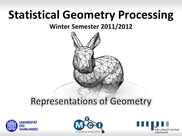
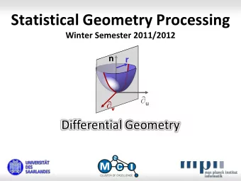
Statistical Geometry Processing Winter Semester 2011/2012 - PowerPoint PPT Presentation

Statistical Geometry Processing Winter Semester 2011/2012 Representations of Geometry

Motivation

Geometric Modeling What do we want to do? empty space  d (typically  3 ) B geometric object B   3 3

Fundamental Problem The Problem:  d B infinite number of points my computer: 8GB of memory We need to encode a continuous model with a finite amount of information 4

Modeling Approaches Two Basic Approaches • Discrete representations  Fixed discrete bins • “Continuous” representations  Mathematical description  Evaluate continuously 5

Discrete Representations You know this... • Fixed Grid of values: ( i 1 , ..., i ds )   ds  ( x 1 , ..., x dt )   dt • Typical scenarios:  d s = 2, d t = 3: Bitmap images  d s = 3, d t = 1: Volume data (scalar fields)  d s = 2, d t = 1: Depth maps (range images) • PDEs: “Finite Differences” models 6

Modeling Approaches Two Basic Approaches • Discrete representations  Fixed discrete bins • “Continuous” representations  Mathematical description  Evaluate continuously 7

Classes of Models Most frequently used models: • Primitive meshes • Parametric models • Implicit models • Particle / point-based models Remarks • Often combinations thereof: hybrid models • Representations can be converted (may be approximate) • Some questions are much easier to answer for certain representations 8

Modeling Zoo

Modeling Zoo Parametric Models Primitive Meshes Implicit Models Point-Based Models 10

Modeling Zoo Parametric Models Primitive Meshes Implicit Models Point-Based Models 11

Parametric Models    ds v S   dt f f ( u , v ) ( u , v ) u Parametric Models • Function f maps from parameter domain  to target space • Evaluation of f gives one point on the model 12

output: 1D output: 2D output: 3D f( t ) t t y t y input: 1D z u x x function graph plane curve space curve y u u y input: 2D z v v x x plane warp surface w y input: 3D u z v x space warp

Modeling Zoo Parametric Models Primitive Meshes Implicit Models Point-Based Models 14

Primitive Meshes Primitive Meshes • Collection of geometric primitives  Triangles  Quadrilaterals  More general primitives (e.g. spline patches) • Typically, primitives are parametric surfaces • Composite model:  Mesh encodes topology, rough shape  Primitive parameter encode local geometry • Triangle meshes rule the world (“triangle soup”) 15

Primitive Meshes  1  2  3 Complex Topology for Parametric Models • Mesh of parameter domains attached in a mesh • Domain can have complex shape (“trimmed patches”) • Separate mapping function f for each part (typically of the same class) 16

Meshes are Great Advantages of mesh-based modeling: • Compact representation (usually) • Can represent arbitrary topology 17

Meshes are not so great Problem with Meshes: • Need to specify a mesh first, then edit geometry • Problems  Mesh structure need to be adjusted to fit shape  Mesh encodes object topology  Changing object topology is painful • Examples  Surface reconstruction  Fluid simulation (surface of splashing water) 18

Triangle Meshes

Triangle Meshes Triangle Meshes: • Triangle meshes: (probably) most common representation • Simplest surface primitive that can be assembled into meshes  Rendering in hardware (z-buffering)  Simple algorithms for intersections (raytracing, collisions) 20

Attributes How to define a triangle? • We need three points in  3 (obviously). • But we can have more: per-vertex normals (represent smooth surfaces more accurately) texture per-vertex texture coordinates per-vertex color (etc...) 21

Shared Attributes in Meshes In Triangle Meshes: • Attributes might be shared or separated: adjacent triangles adjacent triangles share normals have separated normals 22

“Triangle Soup” Variants in triangle mesh representations: • “ Triangle Soup ”  A set S = { t 1 , ..., t n } of triangles  No further conditions  “most common” representation (web downloads and the like) • Triangle Meshes : Additional consistency conditions  Conforming meshes: Vertices meet only at vertices  Manifold meshes: No intersections, no T-junctions 23

Conforming Meshes Conforming Triangulation: • Vertices of triangles must only meet at vertices, not in the middle of edges: • This makes sure that we can move vertices around arbitrarily without creating holes in the surface 24

Manifold Meshes Triangulated two-manifold: • Every edge is incident to exactly 2 triangles (closed manifold) • ...or to at most two triangles (manifold with boundary) • No triangles intersect (other than along common edges or vertices) • Two triangles that share a vertex must share an edge 25

Attributes In general: • Vertex attributes:  Position (mandatory)  Normals  Color  Texture Coordinates • Face attributes:  Color  Texture • Edge attributes (rarely used)  E.g.: Visible line 26

Data Structures The simple approach: List of vertices, edges, triangles v 1 : (posx posy posy), attrib 1 , ..., attrib nav ... v nv : (posx posy posy), attrib 1 , ..., attrib nav e 1 : (index 1 index 2 ), attrib 1 , ..., attrib nae ... e ne : (index 1 index 2 ), attrib 1 , ..., attrib nae t 1 : (idx 1 idx 2 idx 3 ), attrib 1 , ..., attrib nat ... t nt : (idx 1 idx 2 idx 3 ), attrib 1 , ..., attrib nat 27

Pros & Cons Advantages: • Simple to understand and build • Provides exactly the information necessary for rendering Disadvantages: • Dynamic operations are expensive:  Removing or inserting a vertex  renumber expected edges, triangles • Adjacency information is one-way  Vertices adjacent to triangles, edges  direct access  Any other relationship  need to search  Can be improved using hash tables (but still not dynamic) 28

Adjacency Data Structures Alternative: • Some algorithms require extensive neighborhood operations (get adjacent triangles, edges, vertices) • ...as well as dynamic operations (inserting, deleting triangles, edges, vertices) • For such algorithms, an adjacency based data structure is usually more efficient  The data structure encodes the graph of mesh elements  Using pointers to neighboring elements 29

First try... Straightforward Implementation: • Use a list of vertices, edges, triangles • Add a pointer from each element to each of its neighbors • Global triangle list can be used for rendering Remaining Problems: • Lots of redundant information – hard to keep consistent • Adjacency lists might become very long  Need to search again (might become expensive)  This is mostly a “theoretical problem” (O(n) search) 30

Less Redundant Data Structures Half edge data structure: • Half edges, connected by clockwise / ccw pointers • Pointers to opposite half edge • Pointers to/from start vertex of each edge • Pointers to/from left face of each edge 31

Implementation // a half edge // a vertex struct HalfEdge { struct Vertex { HalfEdge * next ; HalfEdge * someEdge ; HalfEdge * previous ; /* vertex attributes */ HalfEdge * opposite ; }; Vertex * origin ; // the face (triangle, poly) Face * leftFace ; struct Face { EdgeData * edge ; HalfEdge* half; }; /* face attributes */ }; // the data of the edge // stored only once struct EdgeData { HalfEdge * anEdge ; /* attributes */ }; 32

Implementation Implementation: • The data structure should be encapsulated  To make sure that updates are consistent  Implement abstract data type with more high level operations that guarantee consistency of back and forth pointers • Free Implementations are available, for example  OpenMesh  CGAL • Alternative data structures: for example winged edge (Baumgart 1975) 33

Modeling Zoo Parametric Models Primitive Meshes Implicit Models Point-Based Models 34

Particle Representations Point-based Representations • Set of points • Points are (irregular) sample of the object • Need additional information to deal with “the empty space around the particles” additional assumptions 35

Meshless Meshes... Point Clouds • Triangle mesh without the triangles • Only vertices • Attributes per point per-vertex normals per-vertex color 36

Particle Representations Helpful Information • Each particle may carries a set of attributes  Must have: Its position  Additional geometry: Density (sample spacing), surface normals  Additional attributes: Color, physical quantities (mass, pressure, temperature), ... • Addition information helps reconstructing the geometric object described by the particles 37

The Wrath of Khan Why Star Trek is at fault... • Particle methods: first used for fuzzy phenomena (fire, clouds, smoke) • “ Particle Systems — a Technique for Modeling a Class of Fuzzy Objects ” [Reeves 1983] • Movie: Genesis sequence 38

Geometric Modeling 3D Scanners • 3D scanner yield point clouds  Have to deal with points anyway • Algorithms that directly work on “point clouds” Data: [IKG, University Hannover, C. Brenner] 39

Modeling Zoo Parametric Models Primitive Meshes Implicit Models Point-Based Models 40