State Estimation for Continuous-Time Systems with Perspective - PDF document

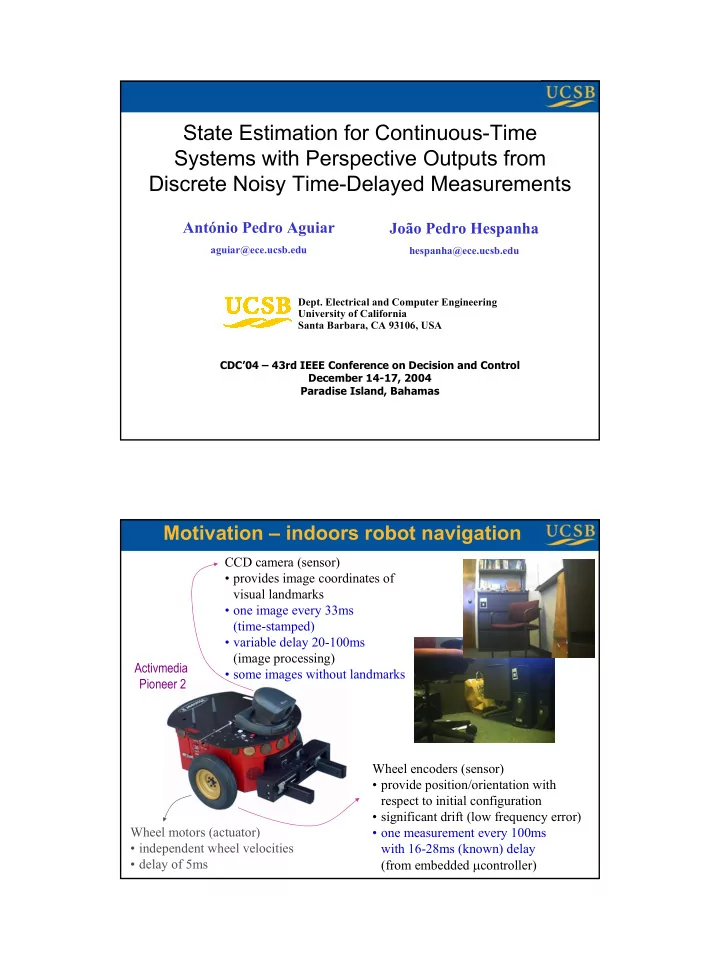
State Estimation for Continuous-Time Systems with Perspective Outputs from Discrete Noisy Time-Delayed Measurements António Pedro Aguiar João Pedro Hespanha aguiar@ece.ucsb.edu hespanha@ece.ucsb.edu Dept. Electrical and Computer Engineering University of California Santa Barbara, CA 93106, USA CDC’04 – 43rd IEEE Conference on Decision and Control December 14-17, 2004 Paradise Island, Bahamas Motivation – indoors robot navigation CCD camera (sensor) • provides image coordinates of visual landmarks • one image every 33ms (time-stamped) • variable delay 20-100ms (image processing) Activmedia • some images without landmarks Pioneer 2 Wheel encoders (sensor) • provide position/orientation with respect to initial configuration • significant drift (low frequency error) Wheel motors (actuator) • one measurement every 100ms • independent wheel velocities with 16-28ms (known) delay • delay of 5ms (from embedded µ controller) 1

Motivation – landing on vision acquire site CCD IR camera (sensor) • provides image coordinates of landing strip • one image every 33ms (time-stamped) • variable delay • landing strip not on all images Inertial sensor & GPS • GPS provides position with respect to earth coordinate system (low sampling rate) • INS provides data at high sampling rate-frequency data with significant Frog UAV (I. Kaminer, NPS) drift (low frequency error) Outline • Systems with perspective outputs • State estimation – The observer equations – Estimator convergence • Pose estimation of autonomous vehicles using CCD cameras • Simulation and Experimental results – Experimental setup – Motion estimation – Output feedback control (parking experiment) 2

Process model State-affine system with multiple perspective outputs disturbance input (cannot be measured) scalar j th perspective measurement inspired by the (single output noise output) perspective – Normalization constraint (specifies α j ) systems introduced by Ghosh et al JMSEC’94 constant vector This system can describe the kinematic model of a rigid-body whose outputs are the (homogeneous) image coordinates of N fixed points provided by an on-board camera. Process model State-affine system with multiple perspective outputs disturbance input (cannot be measured) scalar j th perspective measurement output noise – Normalization constraint (specifies α j ) – Discrete & time-delayed measurements delay discrete measurement generally a strict subset because not all measurements are available simultaneously 3

Process Model State-affine system with multiple discrete & delayed perspective outputs scalar j th discrete & delayed perspective output state-transition matrix of Problem statement State-affine system with multiple discrete & delayed perspective outputs scalar j th discrete & delayed perspective output Goal: Design an optimal observer to estimate the continuous time state vector x ( t ), given the discrete time-delay measurements y j ( t i ). 4

Minimum-energy state-estimation State-affine system with multiple discrete & delayed perspective outputs scalar j th discrete & delayed perspective output Minimum-energy state estimator [Mortensen’68] state value for which the measured outputs can be made compatible with the system dynamics for the “smallest” noise and disturbance in purely continuous or discrete-time gives rise to Kalman-like filter… The observer equations The exact estimate of the state is obtained as the solution to the impulse system Proof: Show that the cost to be minimized can be written as follows… piecewise constant 5

Estimator convergence Problem: Under what conditions the state estimate converges to the true state x • Assuming that P − 1 remains uniformly bounded, there exist positive constants c , r < 1, γ d , γ 1 , ... γ N such that ISS-like bound state estimation error • P − 1 remains uniformly bounded provided that there exist positive constants N , ε such that trajectory-dependent state transition matrix of grammian Vehicle motion estimation using vision Goal: estimate the position & orientation of autonomous vehicle using onboard CCD camera that observes the apparent image motion of stationary points. homogeneous image coordinates of the point Q j ( q b ≡ body, q i ≡ inertial) kinematics configuration of the body frame with respect to the camera frame camera intrinsic parameters The position can be estimated using 6

Experimental results • Pioneer 2-DXE mobile robot from ActivMedia Visual landmark – two front wheels powered by Q 1 Q 2 independent reversible-DC motors – one passive rear caster Q 4 Q 3 – Sony EVI D30 pan-tilt-zoom (PTZ) color video camera Simulation results Following a circular path experiment 4 5 4 x estimation error 2 x error [m] (P) 3 σ min [ P ] 0 σ min 2 -2 0 20 40 60 80 100 120 140 160 180 200 1 time [s] 0 0 0 20 40 60 80 100 120 140 160 180 200 y estimation error time [s] y error [m] -2 50 -4 40 -6 30 (P) 0 20 40 60 80 100 120 140 160 180 200 σ max time [s] 20 1 σ max [ P ] z estimation error 0.5 10 z error [m] 0 0 0 20 40 60 80 100 120 140 160 180 200 time [s] -0.5 1 -1 0 20 40 60 80 100 120 140 160 180 200 measurements available time [s] 0.5 30 0 θ error [degree] σ 20 -0.5 θ estimation error -1 no measurements 10 -1.5 0 -2 0 20 40 60 80 100 120 140 160 180 200 0 20 40 60 80 100 120 140 160 180 200 time [s] time [s] The vision sampling interval is T = 0.4s and the time-delay is τ = 0.2s. The estimation errors only reduce when the visual landmarks are in the camera's field of view. 7

Experimental results Following a circular path experiment measurements 2 σ min [ P ] 400 min (P) Point 1 1 200 σ 0 0 0 50 100 150 200 0 50 100 150 200 1000 σ max [ P ] 400 time [s] time [s] max (P) Point 2 500 200 σ 0 0 0 50 100 150 200 0 50 100 150 200 100 300 time [s] time [s] pan angle 200 Point 3 0 100 -100 0 0 50 100 150 200 0 50 100 150 200 1.5 300 time [s] time [s] 1 200 Point 4 0.5 γ 100 0 -0.5 0 0 50 100 150 200 0 50 100 150 200 time [s] time [s] x estimate 1 x hat [m] 0 -1 0 50 100 150 200 1 time [s] 0 y hat [m] y estimate -1 -2 0 50 100 150 200 0.5 time [s] z hat [m] z estimate 0 0 50 100 150 200 200 time [s] θ estimate 0 θ hat -200 0 50 100 150 200 time [s] Output feedback control (experimental results) 0 Parking experiment -0.5 x [m] x estimate -1 -1.5 0 10 20 30 40 50 60 time [s] 1 y estimate 0.5 y [m] 0 0.1 -0.5 0 10 20 30 40 50 60 time [s] 2 z estimate 0 1 z [m] 0 -1 -0.1 0 10 20 30 40 50 60 time [s] 1 y [m] 0 θ [rad] θ estimate -0.2 -1 -2 0 10 20 30 40 50 60 -0.3 time [s] 0.08 -0.4 0.06 left wheel velocity u 1 [m/s] 0.04 0.02 -0.5 0 0 10 20 30 40 50 60 0 0.1 0.2 0.3 0.4 0.5 0.6 0.7 0.8 time [s] 0.1 x [m] 0.05 u 2 [rad/s] 0 right wheel velocity -0.05 -0.1 -0.15 Minimum-energy state estimator & 0 10 20 30 40 50 60 time [s] 20 pan controller & point stabilization controller camera pan angle 10 pan [degree] 0 (Aicardi et al , IEEE Rob. & Autom. Mag., 95). -10 -20 -30 0 10 20 30 40 50 60 time [s] 8

Conclusions � We addressed the position/orientation estimation for autonomous vehicles using onboard cameras that observe the apparent motion of stationary points (landmarks). � We formulated the problem in the framework of state estimation of a system with perspective outputs with measurements are noisy , arrive at discrete-time instants, suffer delays , and may not be complete . � We designed a dynamical impulsive system that produces an estimate of the state that is “most compatible” with the dynamics, in the sense that it requires the least amount of noise energy to explain the measured output. � The convergence of the proposed estimator system was analyzed and illustrated through computer simulation and experimentally . 9