Last Time TODO add: Estimating worst case execution time PID - - PDF document

1

TODO add: PID material from Pont slides Some inverted pendulum videos Model-based control and other more sophisticated

controllers?

More code speed issues – perf with and w/o FP on

different processors

Last Time

Estimating worst case execution time Holistic scheduling: real-time guarantees over a CAN

bus

Today

Feedback (closed loop) control and PID controllers

Principles Implementation Tuning

Control Systems

Definitions:

Desired state variables: X*(t)

• These are given to the system from outside
• E.g. “room temperature should be 70”

Estimated state variables: X’(t)

• E.g. “room temperature is currently 67”
• Estimation uses standard data acquisition techniques

– E.g. thermistor + ADC

Actions: U(t)

• System commands U(t) converted into driving forces

using transducers

• E.g. “turn off the furnace”

More Control Terms

Goal of a control system is to minimize error:

e(t) = | X*(t) – X’(t) |

Evaluating a control system

Steady-state controller error

• Average e(t)

Transient response

• How long the system takes to reach 99% of the desired

final value after X*(t) is changed

Stability

• Does the system reach a steady state (smooth constant
• utput) or does it oscillate?

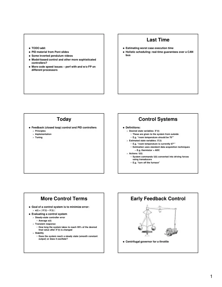
Early Feedback Control

Centrifugal governor for a throttle

2

Simple Closed Loop Example

We’re designing a thermostat

Goal is to heat room to a set temperature We can turn the furnace on and off When furnace is off, room cools down by itself

Fancy control is not needed here! Rather we just need two temperature settings

Tlow – temperature at which we turn on the furnace Thigh – temperature at which we turn off the furnace The difference between these provides hysteresis

An on/off (“bang bang”) controller works well when

the physical system is slow to respond

What happens if control loop runs too fast or slow?

Thermostat Code

int Thigh, Tlow; bool on = false; timer_interrupt_handler (void) { int T = read_adc(); if (T < Tlow && !on) { turn_furnace_on();

• n = true;

} if (T > Thigh && on) { turn_furnace_off();

• n = false;

} }

Another Simple Controller

We’re controlling a robot arm attached to a stepper

motor

Need to get the arm to a certain position Position sensor tells us where the arm is

Algorithm:

if E > 1mm then decrement position by 1mm if E < -1mm then increment position by 1mm

Pretty tough to go wrong with a strategy like this

But slow to converge

What happens if control loop runs too fast or slow?

PID Controllers

Simple controllers like previous two examples work

but in many real situations

Respond slowly Have large errors

Better answer: PID (Proportional Integral Derivative) PID equation: KP, KI, and KD are design parameters

Can be fixed at zero to simplify the controller

dt t dE K d E K t E K t U

t D I P

) ( ) ( ) ( ) (

• +

+ = τ τ

PID Intuition

KP – determines response to current error

Too large Oscillation Too small Slow response Can’t eliminate steady-state error

KI – determines response to cumulative error

Can eliminate steady-state error but often makes transient

response worse

KD – determines response to rate of change of error

Damps response when error is moving in the right

direction

Amplifies response when error is moving in the wrong

direction

Can be used to increase stability and improve transient

response

PID Loop Skeleton Code

double UpdatePID (SPid *pid, double error, double position) { … } position = ReadPlantADC(); drive = UpdatePID (&plantPID, plantCommand - position, position); DrivePlantDAC (drive);

3

Proportional Control

double UpdatePID (SPid *pid, double error, double position) { double pTerm; pTerm = pid->pGain * error; return pTerm; }

Example System 1 Example System 2

Problem: Proportional control can’t always eliminate

steady-state error

Example System 3

Problem: When there is too much actuator delay,

proportional control cannot stabilize the system

Integral Control

double iTerm; pid->iState += error; if (pid->iState > pid->iMax) { pid->iState = pid->iMax; } else if (pid->iState < pid-> iMin) { pid->iState = pid->iMin; } iTerm = pid->iGain * iState;

In practice, always used in conjunction with

proportional control

Example 2 with PI Control

Steady state error is eliminated

4

Integrator Issues

Sampling time becomes more important

Sampling time shouldn’t vary more than 1%-5% On average, sampling should be periodic

Integrator range is important

“Integrator windup” occurs when the integrator value gets

stuck too high or too low

Limiting the range makes this less of a problem Reasonable heuristic: Set integrator limits to drive limits

Usually, if you can’t stabilize a system with

proportional control, you can’t stabilize it with PI control either

Differential Control

double dTerm; dTerm = pid->dGain * (position - pid->dState); pid->dState = position;

Basically just computes the slope of the system

state

Attempts to predict system future based on recent

past history

Example 3 with PD Control Differential Issues

Derivative is very sensitive to noise

In practice, might keep a buffer of several samples into the

past in order to smooth out noise

• This is just a low-pass filter
• Decreases responsiveness – which is the point of

differential control in the first place

Important for sampling period to be very even

Do sampling in a high-priority interrupt or thread

Full PID Source Code

typedef struct { double dState; // Last position input double iState; // Integrator state double iMax, iMin; double iGain, // integral gain pGain, // proportional gain dGain; // derivative gain } SPid; double UpdatePID (SPid * pid, double error, double position) { double pTerm, dTerm, iTerm; pTerm = pid->pGain * error; pid->iState += error; if (pid->iState > pid->iMax) pid->iState = pid->iMax; else if (pid->iState < pid->iMin) pid->iState = pid->iMin; iTerm = pid->iGain * iState; dTerm = pid->dGain * (position - pid->dState); pid->dState = position; return pTerm + iTerm - dTerm; }

Implementation Issues

Example code uses floating point

Convert to integer or fixed-point by hand

OR

Keep using FP if the control loop frequency is low or if HW

FP is available

Multiplies can be avoided by selecting constants that

are multiples of 2

Sampling rate

Too low Slow response time Too high Differential noise and integral overflow Rule of thumb: Set sampling rate between 1/10 and 1/100 of

desired settling time

Difficult control problems argue for higher sampling rates

5

Tuning the Parameters

Method 1: Plug system model into Matlab, it hands

you the parameters

Method 2: Tune by hand

Happy fact: When the system is not too sensitive, control

parameters only have to be roughly correct to do a good job

Requirements for hand tuning:

Need to be able to observe controller variables and output Need to be able to supply square-wave inputs

Note: Parameters can interact in complex ways

Tuning is an art Tuning by hand will be difficult if system is barely

controllable

System may be uncontrollable

Tuning Differential Gain

Start here unless you can do without dGain, in which

case set it to 0.0 and move to pGain

Start with small proportional gain, e.g. 1.0 Start with dGain == pGain * 100 Increase dGain until unacceptable oscillation,

• vershoot, or noise occurs

Oscillation from too much dGain is much faster than

• scillation from not enough

Back off by factor of 2-4 System will now be sluggish – time to tune P and I

Tuning pGain and iGain

Start with a pGain around 1-100 By experimentation find the value of pGain where

• scillation starts

Then back off by a factor of 2-4 Start with iGain around 0.0001-0.001 Again find a value that gives reasonably good

performance without causing oscillation

Conclusions

Feedback control is a broadly useful technology for

getting an embedded system to have some desired effect on the real world

In practice manual tuning replaces analytic solutions However, Matlab has great support for feedback

control

Can generate efficient code too