
SLIDE 1
Transform´ ee de Riesz multi-´ echelles et Applications ` a l’image 1
Val´ erie Perrier
Laboratoire Jean Kuntzmann Universit´ e de Grenoble-Alpes
Collaborateurs : Marianne Clausel, Sylvain Meignen, K´ evin Polisano (LJK), Laurent Desbat (TIMC-Imag) and Thomas Oberlin (IRIT, Toulouse)
- 1. Journ´
ee ” Temps-Fr´ equence et Non-Stationnarit´ e” , Marseille, 19 juin 2015
1
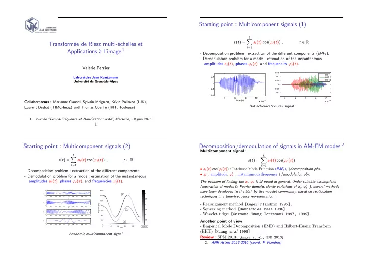
Starting point : Multicomponent signals (1)
s(t) =
L
- ℓ=1
aℓ(t) cos(ϕℓ(t)) , t ∈ R
- Decomposition problem : extraction of the different components (IMFℓ).
- Demodulation problem for a mode : estimation of the instantaneous
amplitudes aℓ(t), phases ϕℓ(t), and frequencies ϕ′
ℓ(t).
4 6 8 10 x 10
−3
−0.2 −0.1 0.1 time (s) 2 4 6 8 10 x 10
−3
−0.1 −0.05 0.05 0.1 0.15 IMF 1 IMF 2 IMF 3
Bat echolocation call signal
Starting point : Multicomponent signals (2)
s(t) =
L
- ℓ=1
aℓ(t) cos(ϕℓ(t)) , t ∈ R
- Decomposition problem : extraction of the different components.
- Demodulation problem for a mode : estimation of the instantaneous
amplitudes aℓ(t), phases ϕℓ(t), and frequencies ϕ′
ℓ(t).
0.1 0.2 0.3 0.4 0.5 0.6 0.7 0.8 0.9 1 −10 10 t s 0.1 0.2 0.3 0.4 0.5 0.6 0.7 0.8 0.9 1 −5 5 t s1 0.1 0.2 0.3 0.4 0.5 0.6 0.7 0.8 0.9 1 −2 2 t s2 0.1 0.2 0.3 0.4 0.5 0.6 0.7 0.8 0.9 1 −2 2 t s3
0.2 0.4 0.6 0.8 1 20 40 60 80 100 120 140 time frequency (Hz) 0.5 1 1.5 2 2.5 3 s3 s2 s1
Amplitude
Academic multicomponent signal
Decomposition/demodulation of signals in AM-FM modes 2
Multicomponent signal : s(t) =
L
- ℓ=1
aℓ(t) cos(ϕℓ(t))
- aℓ(t) cos(ϕℓ(t)) : Intrinsec Mode Function (IMFℓ), (decomposition pb).
- aℓ : amplitude, ϕ′
ℓ : instantaneous frequency (demodulation pb).
The problem of finding the aℓ, ϕℓ is ill-posed in general. Under suitable assumptions (separation of modes in Fourier domain, slowly variations of a′
ℓ, ϕ′ ℓ..), several methods
have been developed in the 90th by the wavelet community, based on reallocation techniques in a time-frequency representation :
- Reassignment method [Auger-Flandrin 1995],
- Squeezing method [Daubechies-Maes 1996],
- Wavelet ridges [Carmona-Hwang-Torr´
esani 1997, 1999]. Another point of view :
- Empirical Mode Decomposition (EMD) and Hilbert-Huang Transform