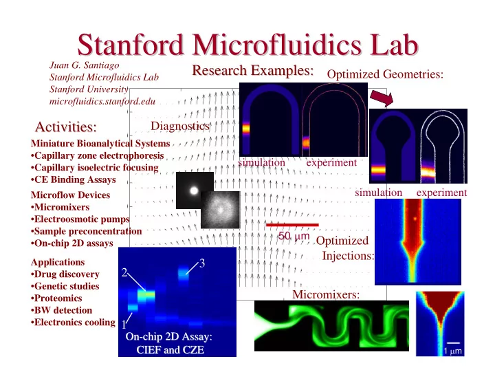
stanford microfluidics microfluidics lab lab stanford
play

Stanford Microfluidics Microfluidics Lab Lab Stanford Juan G. - PowerPoint PPT Presentation

Stanford Microfluidics Microfluidics Lab Lab Stanford Juan G. Santiago Research Examples: Research Examples: Optimized Geometries: Stanford Microfluidics Lab Stanford University microfluidics.stanford.edu Activities: Diagnostics


  1. Stanford Microfluidics Microfluidics Lab Lab Stanford Juan G. Santiago Research Examples: Research Examples: Optimized Geometries: Stanford Microfluidics Lab Stanford University microfluidics.stanford.edu Activities: Diagnostics Activities: Miniature Bioanalytical Systems • Capillary zone electrophoresis simulation experiment • Capillary isoelectric focusing • CE Binding Assays simulation experiment Microflow Devices • Micromixers • Electroosmotic pumps • Sample preconcentration 50 µ m Optimized • On-chip 2D assays Injections: Applications 3 2 • Drug discovery • Genetic studies Micromixers: • Proteomics • BW detection • Electronics cooling 1 On- On -chip 2D Assay: chip 2D Assay: 1 µ m CIEF and CZE CIEF and CZE

  2. Electrokinetics Microfluidics at Extreme Scales 10 µm 10 µm Juan G. Santiago Stanford Microfluidics Laboratory Mechanical Engineering Department Stanford University

  3. Outline (time, concentration, length) • Introduction � Microfluidics � Electrokinetic (EK) flows • Electrokinetic instabilities (time) � Mechanism and model � Transition to chaos • ITP (concentration) � Sensitivity and practice � Extreme concentration scales • Nanochannel electrophoresis (length) � Small ion separations � DNA sample separation � Near-Future Work

  4. Microfluidics • Applications � Point-of-care medical diagnostics � Bio-weapon detection � Pharmaceuticals/drug discovery � Environmental monitoring Image courtesy www.calipertech.com • Challenges and Advantages � Reduced reagent use � Specificity, robustness 0.7 cm � Portability vs. sensitivity � Integration and automation � Potential for parallel analyses www.nanogen.com

  5. Processes in microfluidics ≠ ∇ > u u i u 0 drift ,1 drift ,2 drift Separation Stacking Hybridization Reaction

  6. Separation in H-filter ∆ • diffusivity uFluidics ∆ • mobility On-chip CE ∆ • valence Nanochannel electrophoresis ≠ u u ∆ drift ,1 drift ,2 • affinity ∆ • polarizability ∇ ∆ • size/steric force

  7. Electroosmotic flow Wall u(y) External Electric Field y x Wall y • Zeta vs. chemistry? λ D • EDL overlap? shear plane • Condensation? ζ ψ adsorbed ion

  8. Electrohydrodynamics and Electrokinetics History Reuss, F.F. 1809. Memoires de ls Societe Imperial des Naturalistes de Moscow. 2:327. Gilbert, ~1580s Of the attraction exerted by amber

  9. Electrokinetic Microfluidics 100 um λ d + + Pressure-driven Electrokinetic Glass or fused-silica microchannel wall + + + + + + + + + + + EOF - - + + - + - Electrophoresis + - + λ d Charge + + + + + λ d + double-layer + + + + + ++ + + + + Devasenathipathy S. and J. Santiago, Micro- Deprotonated silanol groups and nano-scale diagnostics , Springer-Verlag, 2003 • Electric control (no moving parts) • Switching, valving • Low dispersion • Integrated w/ separation techniques 100 um

  10. Electrokinetic Instabilities

  11. Complex electrokinetics • Sample preconcentration methods � Thermal gradient focusing � Field amplified sample stacking � Isotachophoresis 6 3 • On-chip two-dimensional assays CE dimension (mm) 5 2 1 B 4 Signal (au) 3 2 1 A C 1 D 0 IEF/EOF ∆ x = 4 W IEF dimension (mm) Herr, A.E. et al. Analytical Chemistry , Vol. 75, No. 5, pp. 1180-1187, 2003 • On-chip CE with unknown or poorly controlled sample chemistry • On-chip mixing and buffer exchange

  12. Major Challenge in Heterogenous Particle visualization EK Systems: Instabilities Flows at Intersections: Axial interface: 1 mm 50 µ m Unstable, fluctuating concentrations in high- conductivity-gradient case 100 µ m 100 µ m

  13. EK Instability Mechanism σ L σ L σ L Ε L σ L σ L σ L - - - σ H σ H +++ σ H σ H σ H σ H Ε H σ L Ε H Ε L σ L σ H σ L σ H σ L σ H σ H

  14. Electrokinetic Flow Instabilities depth d • Generated by net charge in bulk δ σ L Ε L - - - Ε H ρ ≅ ε ⋅∇ σ σ ∆ / ~ E C +++ � E ε E E H σ H EV = L a U � Velocity scale: µ ε γ − 2 2 U d E d 1 ∗ ∗ ≡ = ∇ σ ev 0 � Controlling parameter: Ra � µ γ , e D D max ε γ − γδ ∆ − − − E 0 ( 1) / F 5 6 • C scales as ~ 10 10 0 • EOF coupling produces convective instab. • Multiple ion mobilities have severe impact Diffusion Electromigration ��� � ��� � � ����� χ σ 1 D ∑ ∑ = ∇ + ∇⋅ ∇ φ j 2 c ( c ) j j Oddy and Santiago, in press, Physics of Fluids , 2005. Dt Pe Pe j j j j Posner and Santiago, J. of Fluid Mechanics , pp. 1-42, 2006. Chen, C.-H. et al., J. of Fluid Mechanics , 524, pp. 263 – 303, 2005. Lin, H. et al., Vol. 16, No. 6 Physics of Fluids , p.1922-1935, 2004. 0

  15. Electrokinetic instabilities t = 0.0 s t = 0.5 s t = 1.0 s t = 1.5 s t = 2.0 s t = 2.5 s t = 3.0 s t = 4.0 s t = 5.0 s Model Experiment Storey, B.D. et al. Physics of Fluids , Vol. 16, No. 6, p.1922-1935, 2004. Lin et al., submitted to J. Fluid Mechanics , 2005.

  16. EKI in a cross intersection: Experiments Power spectra Ra e = 675 50 um Ra e = 800 Ra e = 2,000 Ra e = 2,700 f [1/sec]

  17. Temporal Power Spectrum Ra e f [1/sec]

  18. Correlation plots C1 Ra e =675 Ra e =800 C1 Ra e =2000 Ra e =2600 C2 C2

  19. Isotachophoresis

  20. ITP History • Kohlrausch : KRF function in 1897. • Tiselius : Moving boudnary electrophoresis, 1930 • Longsworth : Performed moving boundary electrophoresis in 1939. • Martin AJP: Displacement electrophoresis (also called ITP) in 1942 for cation. • Everaerts and Martin: First to perform ITP in thin capillaries (200 to 500 micron) in 1963. Used HEC to suppress EOF.

  21. Detection Microchip/ Method Sample Electrolyte SE Comments Ref. Mode capillary didansyl-lysine Sodium tetraborate (0.5 First on-chip FASS FASS Fluore- Microchip 13.8 1995 mM and 500 mM) Run-time: 20 sec scence Carbonate (200 μ M and 32 Fluore- Microchip FITC-arginine 65 Six-channel geometry FASS 2001 mM) Run-time: 2 min scence Microchip Fluorescein sodium HEPES (0.1 mM and 100 100 Five-channel geometry. FASS Fluore- 2003 salt mM), NaCl (0.2 mM and Run-time: 1 min. scence 200 mM) Fluore- Microchip Fluorescein 175 mM Phosphate, DI 80 Narrow sample channel FASS 2003 disodium salt water Run-time: 2 min scence eTags LE: 25 mM imidazole, 20 Run-time: 1-2 min ITP Fluore- Microchip 530 2002 mM HCl, TE: 160 mM scence imidazole, 40 mM HEPES Microchip Fluorescein LE: 250 mM NaCl, TE: 95 500 Run-time: 2 min ITP Fluore- 2005 mM TAPS, 73 mM TEA scence PTH-aspartic acid, 100 mM MES and 100 mM First LVSS LVSS UV Capillary - 1992 PTH-glutamine acid histidine, DI water Run-time: 6-10 min L d) = 65 cm Dese, Amino 45 mM NaH 2 PO 4 and 15 Run-time: 4-6 min FASS UV Capillary 1000 1996 mM Na 2 HPO 4 , 60% v/v L = 24.6 cm 1 - propanol Maleic, fumaric 1 mM phosphoric acid, 40 Run-time: 5-10 min LVSS UV Capillary 300 1999 acids, bromide, mM potassium dihydrogen L = 61 cm nitrate phosphate 75 mM phosphate, DI water Run-time: 15-17 min FASI UV Capillary Bromide, nitrate, 1000 1999 bromate L = 25 cm 1 - naphthylamine, 50 mM phosphoric acid Run-time: 10-13 min FASI UV Capillary 200 2000 laudanosine with 20 % acetonitrile, DI L = 64 cm water NXX-066 LE: 10 mM NaOH titrated Highest ITP stacking ITP UV Capillary 5500 1998 with H 3 PO 4 , TE: 6.13 mM Run-time: 6-10 min L = 53.5 cm THeACl titrated with H 3 PO 4

  22. Sensitivity in Capillary Electrophoresis (no stacking) 1.E-02 UV absorbance indirect fluorescence thermooptical end-column detection absorbance electrochemical detection 1.E-04 concentration (mol/l) mass spectrometric detection conductivity detection 1.E-06 UV absorbance with Z-shaped flow cells amperometric UV absorbance detection detection 1.E-08 Belder et al. electrochemical (2002) detection 1.E-10 Chen et al. radiochemical (1996) detection conductivity detection 1.E-12 with ITP stacking Ocvirk et al. fluorescence (1998) detection 1.E-14 1E-23 1E-21 1E-19 1E-17 1E-15 1E-13 1E-11 molar sensitivity (mol)

  23. Single Interface Isotachophoresis E E Order of mobility Leading Ion (LE) ν > ν ν > Sample Ion • Characteristics Trailing Ion (TE) Sample zone grows with time. Counterion not shown � Stable concentration boundaries � Final Sample Concentration depends on Leading ion concentration �

  24. ITP (S - ) Alexa fluor (1 µ M) HEPES (5mM)(TE) HEPES (5mM) NaCl (large excess) (LE) 50 µ m γ = 393 • Concentration enhancement greater than γ • Buffer selections allow for both ITP and FASS • ITP-type stacking with CE separation

  25. Stable over 1000+ diameters Stable across flow geometries 50 µ m 5 mm Stability under large disturbances 50 µ m

Download Presentation
Download Policy: The content available on the website is offered to you 'AS IS' for your personal information and use only. It cannot be commercialized, licensed, or distributed on other websites without prior consent from the author. To download a presentation, simply click this link. If you encounter any difficulties during the download process, it's possible that the publisher has removed the file from their server.

Recommend


More recommend