Stability of Cluster Analysis 2. Preparation of the data 3. Distance - - PowerPoint PPT Presentation

SLIDE 1

Stability of Cluster Analysis

S T A T I S T I K A U S T R I A

D i e I n f o r m a t i o n s m a n a g e r

Matthias Templ & Peter Filzmoser

Vienna University of Technology Vienna, June 16, 2006

Stability of Cluster Analysis

For real data sets without obvious grouping structure the stability of clusters depends on:

• 1. Input data - the selection of variables
• 2. Preparation of the data
• 3. Distance measure used ∗
• 4. Clustering method
• 5. Number of clusters

Changing one parameter may result in complete different cluster results.

∗if a distance measure must be chosen

• 1. Input Data - Variable Selection

> library(mvoutlier) > library(cluster) > data(humus) > a <- agnes(t(prepare(humus[, -c(1:3)]))) > plot(a, which.plots = 2, col = c(4), col.main = 3, col.sub = 2)

• 1. Input Data - Variable Selection

> library(mvoutlier) > data(humus) > a <- agnes(t(prepare(humus[, -c(1:3)]))) > plot(a, which.plots = 2, col = c(4), col.main = 3, col.sub = 2)

Ag Bi Pb Rb Tl Ba Si K Mn Zn Al Be La Y Th U Cr V Fe Sc As Co Cu Ni Mo Cd P B Mg Na pH Ca Sr Hg S N C H LOI Sb Cond 5 10 15 20 25 30 35

Dendrogram of agnes(x = t(prepare(humus[, −c(1:3)])))

Agglomerative Coefficient = 0.47 t(prepare(humus[, −c(1:3)])) Height

A chemical process can be seen in more detail in a map (later) by choosing similar variables.

SLIDE 2

• 1. Input Data - Variable Selection

A selection of variables may be useful when clustering high-dimensional data because . . .

• clustering with all variables may hide underlying processes
• we want to see some processes in more detail
• the inclusion of one irrelevant variable may hide the real clusters in the data

One easy way (amongst others) for variable selection can be done by graphical inspection

• f a dendrogram which results from hierarchical clustering of variables.
• 2. Data Preparation

Most of real data in practice can have some or all of these properties:

• neither normal nor log-normal
• strongly skewed
• often multi-modal distributions
• dependencies between observations
• weak clustering structures
• data includes outliers
• variables show a striking difference in the amount of variability
• 2. Data Preparation

If a good clustering structure for a variable exists we expect a distribution with two or more

• modes. A transformation (e.g with a box-cox transformation) will preserve the modes

but remove large skewness. Standardisation of the variables is needed if the variables show a striking difference in the amount of variability. Outliers can influence the clustering (depends on which clustering algorithms is chosen) Removing outliers before clustering may be useful. Finding outliers is not a trivial task, especially in high dimensions. (you can do this e.g. with Package mvoutlier from Filzmoser et al. (2005))

• 3. Distance Measure

pam.euclidean pam.manhattan pam.gower pam.rf kmeans.euclidean kmeans.manhattan kmeans.gower kmeans.rf 0.2 0.4 0.6 0.8 1.0

Rand Index for 500 bootstrap samples Rand Index

Comparing clustered data and clustered subsets of the data with Rand Index. Distance measures which results in high Rand Indices should be chosen.

SLIDE 3

• 4. Clustering Method

pam.euclidean pam.manhattan pam.gower pam.rf kmeans.euclidean kmeans.manhattan kmeans.gower kmeans.rf 0.2 0.4 0.6 0.8 1.0

Rand Index for 500 bootstrap samples Rand Index

Comparing clustered data and clustered subsets of the data with Rand Index. Algorithms which results in high Rand Indices may be chosen.

• 5. Number of Clusters

number of clusters wb.ratio

2 4 6 8 0.4 0.6 0.8

bclust clara

2 4 6 8

cmeans kccaKmedians

2 4 6 8

Mclust speccPolydot euclidean gower manhattan none rf

Data: HumusCoNiCuAsMo Pollution

• 5. Number of Clusters

number of clusters wb.ratio

2 4 6 8 0.4 0.6 0.8

bclust clara

2 4 6 8

cmeans kccaKmedians

2 4 6 8

Mclust speccPolydot euclidean gower manhattan none rf

Data: HumusCoNiCuAsMo Pollution

− → Example

• bs = 27

separation = 2.02

1

• bs = 35

separation = 2.67

2

• bs = 126

separation = 3.81

3

• bs = 22

separation = 2.46

4

• bs = 74

separation = 2.55

5

• bs = 34

separation = 2.36

6

• bs = 166

separation = 2.02

7

• bs = 100

separation = 2.11

8

• bs = 33

separation = 2.4

9

− →

SLIDE 4

• bs = 27

separation = 2.02

1

• bs = 35

separation = 2.67

2

• bs = 126

separation = 3.81

3

• bs = 22

separation = 2.46

4

• bs = 74

separation = 2.55

5

• bs = 34

separation = 2.36

6

• bs = 166

separation = 2.02

7

• bs = 100

separation = 2.11

8

• bs = 33

separation = 2.4

9 Ag Al As B Ba Be Bi Ca Cd Co Cr Cu Fe Hg K La Mg Mn Mo Na Ni P Pb Rb S Sb Sc Si Sr Th Tl U V Y Zn C H N LO pH Co

1

Ag Al As B Ba Be Bi Ca Cd Co Cr Cu Fe Hg K La Mg Mn Mo Na Ni P Pb Rb S Sb Sc Si Sr Th Tl U V Y Zn C H N LO pH Co

2

Ag Al As B Ba Be Bi Ca Cd Co Cr Cu Fe Hg K La Mg Mn Mo Na Ni P Pb Rb S Sb Sc Si Sr Th Tl U V Y Zn C H N LO pH Co

3

Ag Al As B Ba Be Bi Ca Cd Co Cr Cu Fe Hg K La Mg Mn Mo Na Ni P Pb Rb S Sb Sc Si Sr Th Tl U V Y Zn C H N LO pH Co

4

Ag Al As B Ba Be Bi Ca Cd Co Cr Cu Fe Hg K La Mg Mn Mo Na Ni P Pb Rb S Sb Sc Si Sr Th Tl U V Y Zn C H N LO pH Co

5

Ag Al As B Ba Be Bi Ca Cd Co Cr Cu Fe Hg K La Mg Mn Mo Na Ni P Pb Rb S Sb Sc Si Sr Th Tl U V Y Zn C H N LO pH Co

6

Ag Al As B Ba Be Bi Ca Cd Co Cr Cu Fe Hg K La Mg Mn Mo Na Ni P Pb Rb S Sb Sc Si Sr Th Tl U V Y Zn C H N LO pH Co

7

Ag Al As B Ba Be Bi Ca Cd Co Cr Cu Fe Hg K La Mg Mn Mo Na Ni P Pb Rb S Sb Sc Si Sr Th Tl U V Y Zn C H N LO pH Co

8

Ag Al As B Ba Be Bi Ca Cd Co Cr Cu Fe Hg K La Mg Mn Mo Na Ni P Pb Rb S Sb Sc Si Sr Th Tl U V Y Zn C H N LO pH Co

9

• bs = 27

separation = 2.02

1

• bs = 35

separation = 2.67

2

• bs = 126

separation = 3.81

3

• bs = 22

separation = 2.46

4

• bs = 74

separation = 2.55

5

• bs = 34

separation = 2.36

6

• bs = 166

separation = 2.02

7

• bs = 100

separation = 2.11

8

• bs = 33

separation = 2.4

9 Ag Al As B Ba Be Bi Ca Cd Co Cr Cu Fe Hg K La Mg Mn Mo Na Ni P Pb Rb S Sb Sc Si Sr Th Tl U V Y Zn C H N LO pH Co

1

Ag Al As B Ba Be Bi Ca Cd Co Cr Cu Fe Hg K La Mg Mn Mo Na Ni P Pb Rb S Sb Sc Si Sr Th Tl U V Y Zn C H N LO pH Co

2

Ag Al As B Ba Be Bi Ca Cd Co Cr Cu Fe Hg K La Mg Mn Mo Na Ni P Pb Rb S Sb Sc Si Sr Th Tl U V Y Zn C H N LO pH Co

3

Ag Al As B Ba Be Bi Ca Cd Co Cr Cu Fe Hg K La Mg Mn Mo Na Ni P Pb Rb S Sb Sc Si Sr Th Tl U V Y Zn C H N LO pH Co

4

Ag Al As B Ba Be Bi Ca Cd Co Cr Cu Fe Hg K La Mg Mn Mo Na Ni P Pb Rb S Sb Sc Si Sr Th Tl U V Y Zn C H N LO pH Co

5

Ag Al As B Ba Be Bi Ca Cd Co Cr Cu Fe Hg K La Mg Mn Mo Na Ni P Pb Rb S Sb Sc Si Sr Th Tl U V Y Zn C H N LO pH Co

6

Ag Al As B Ba Be Bi Ca Cd Co Cr Cu Fe Hg K La Mg Mn Mo Na Ni P Pb Rb S Sb Sc Si Sr Th Tl U V Y Zn C H N LO pH Co

7

Ag Al As B Ba Be Bi Ca Cd Co Cr Cu Fe Hg K La Mg Mn Mo Na Ni P Pb Rb S Sb Sc Si Sr Th Tl U V Y Zn C H N LO pH Co

8

Ag Al As B Ba Be Bi Ca Cd Co Cr Cu Fe Hg K La Mg Mn Mo Na Ni P Pb Rb S Sb Sc Si Sr Th Tl U V Y Zn C H N LO pH Co

9 Pollution Highest pollution visualised by cluster 9 This can be seen in the graphic on the right e.g. Co, Cu, Ni typical elements for reflecting pollution Mclust on scaled and transformed humus data Validity measure on each cluster cluster size Visualising all clusters each in an own map Seaspray Cluster 5 (Greyscale depends on validity measure in each cluster)

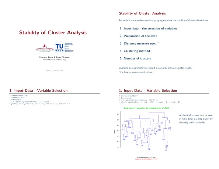
Conclusions

• Applying cluster analysis on real data results in highly non-stable results for many

reasons

• The selection of variables and the selection of the optimal number of clusters on real

data is a non-trivial task.

• Cluster analysis can be seen as explorative data analysis to get ideas about your data
• Interactive tools which allow for various methods are very helpful