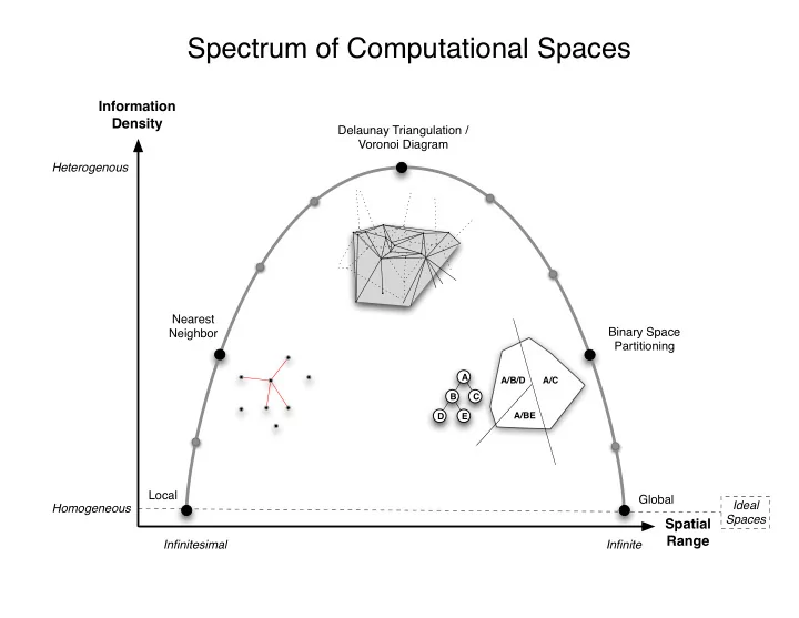
Spectrum of Computational Spaces Information Density Delaunay - PowerPoint PPT Presentation

Spectrum of Computational Spaces Information Density Delaunay Triangulation / Voronoi Diagram Heterogenous Nearest Binary Space Neighbor Partitioning A A/B/D A/C B C A/BE D E Local Global Ideal Homogeneous Spaces Spatial Range Infinitesimal Infinite

Coordinates and Vectors Addition Dot Product Cross Product A A B C |A|*|B|*cos( � ) � B dot(A, B) = |A|*|B|*cos( � ) AxB = C, |C| = |A|*|B|*sin( � ) Subtraction answers the question: answers the questions: How much is a vector aligned with How orthogonal are two vectors? another? What plane do two vectors define?

Rendering Pipeline Geometry Camera Culling Window gluLookAt glPerspective glOrtho glTranslate glFrustum glRotate glVertex glScale glViewport Normalized Object Eye Clip Device Window Coordinates Coordinates Coordinates Coordinates Coordinates Divide by Viewport (x, y, z) (x w , y w, Zw ) ModelView Projection W Transform (x, y, z, 1) (x e , y e , z e , 1) (x c , y c , z c , 1) (x n , y n , z n ) x, y, z � [-1, 1] Transpose(Inverse( MV )) Normal (x, y, z) (x e , y e , z e ) Matrix glNormal

ModelView Matrix X eye X X W eye = = � � � Y eye Y Y M modelview M view M model Z eye Z Z W =1 W =1 Homogeneous Coordinates Canonical Affine Transformation m00 m10 m20 T0 X m00 m10 m20 X T0 m01 m11 m21 T1 Y � � + m01 m11 m21 Y T1 m02 m12 m22 T2 Z m02 m12 m22 Z T2 0 0 0 1 1

glTranslate( Tx, Ty, Tz) ( 0, 0, 0) ( t0, t1, t2) 1 0 0 Tx 0 1 0 Ty 0 0 1 Tz 0 0 0 1 Translation

glRotate( angle, Rx, Ry, Rz) (Rx, Ry, Rz) X angle R00 R10 R20 0 R01 R11 R21 0 R02 R12 R22 0 0 0 0 1 Rotation

Rotation glRotate( � , 0, 0, 1) Y-axis cos( � ) -sin( � ) 0 0 (-sin( � ), cos( � )) sin( � ) sin( � ) cos( � ) 0 0 (cos( � ), sin( � )) Z-axis roll 0 0 1 0 cos( � ) � sin( � ) 0 0 0 1 � X X-axis cos( � ) 0 -sin( � ) 0 cos( � ) 0 1 0 0 Y-axis Yaw -sin( � ) 0 cos( � ) 0 Compound rotation of 3 angles: glRotate( Pitch , 1, 0, 0) 0 0 0 1 glRotate( Yaw , 0, 1, 0) glRotate( Roll , 0, 0, 1) 1 0 0 0 0 cos( � ) -sin( � ) 0 X-axis Pitch 0 sin( � ) cos( � ) 0 0 0 0 1

glScale( Sx, Sy, Sz) s2 s1 s0 Sx 0 0 0 0 Sy 0 0 0 0 Sz 0 0 0 0 1 Scale

Up gluLookAt( eye, center, up ) Look = Center - Eye Left = Up X Look Left Eye Look Center Left(x) Left(y) Left(z) 0 m00 m10 m20 T0 Up(x) Up(y) Up(z) 0 m01 m11 m21 T1 � Look(x) Look(y) Look(z) 0 m02 m12 m22 T2 0 0 0 1 0 0 0 1 Viewing Axes Current MV Note: viewing transforms can be thought of as opposing model transforms, thus the transposed axes in the View Matrix

1D Projective Mapping How to map line L to line M ? Desirable Properties: bijectivity L A' C B/B' A C' M � L � Ideal Point Ideal Point M Eye

Projective Plane (P2): E3 = 3D Euclidean Space P2 = Projective Plane Set of all equivalence classes of ordered triples of non-zero vectors S2 = Unit sphere in E3 in E3 where equivalence is the mutual proportionality of two vectors Set of all lines passing through the origin of E3 ( k x, k y, kz, k w) equivalent points (x, y, z, w) P2 (x/w, y/w, z/w, 1) w=1 w=0 S2 ideal lines

Fundamental Polygons pole A A A B A B pole Möbius Strip Sphere A A B B B B A A Torus Projective Plane