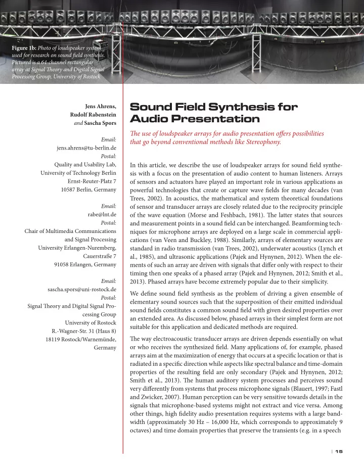
Sound Field Synthesis for Jens Ahrens, Rudolf Rabenstein Audio - - PDF document

| 15

Sound Field Synthesis for Audio Presentation

Te use of loudspeaker arrays for audio presentation offers possibilities that go beyond conventional methods like Stereophony.

In this article, we describe the use of loudspeaker arrays for sound field synthe- sis with a focus on the presentation of audio content to human listeners. Arrays

• f sensors and actuators have played an important role in various applications as

powerful technologies that create or capture wave fields for many decades (van Trees, 2002). In acoustics, the mathematical and system theoretical foundations

• f sensor and transducer arrays are closely related due to the reciprocity principle
• f the wave equation (Morse and Feshbach, 1981). Te latter states that sources

and measurement points in a sound field can be interchanged. Beamforming tech- niques for microphone arrays are deployed on a large scale in commercial appli- cations (van Veen and Buckley, 1988). Similarly, arrays of elementary sources are standard in radio transmission (van Trees, 2002), underwater acoustics (Lynch et al., 1985), and ultrasonic applications (Pajek and Hynynen, 2012). When the ele- ments of such an array are driven with signals that differ only with respect to their timing then one speaks of a phased array (Pajek and Hynynen, 2012; Smith et al., 2013). Phased arrays have become extremely popular due to their simplicity. We define sound field synthesis as the problem of driving a given ensemble of elementary sound sources such that the superposition of their emitted individual sound fields constitutes a common sound field with given desired properties over an extended area. As discussed below, phased arrays in their simplest form are not suitable for this application and dedicated methods are required. Te way electroacoustic transducer arrays are driven depends essentially on what

• r who receives the synthesized field. Many applications of, for example, phased

arrays aim at the maximization of energy that occurs at a specific location or that is radiated in a specific direction while aspects like spectral balance and time-domain properties of the resulting field are only secondary (Pajek and Hynynen, 2012; Smith et al., 2013). Te human auditory system processes and perceives sound very differently from systems that process microphone signals (Blauert, 1997; Fastl and Zwicker, 2007). Human perception can be very sensitive towards details in the signals that microphone-based systems might not extract and vice versa. Among

• ther things, high fidelity audio presentation requires systems with a large band-

width (approximately 30 Hz – 16,000 Hz, which corresponds to approximately 9

• ctaves) and time domain properties that preserve the transients (e.g. in a speech

Jens Ahrens, Rudolf Rabenstein and Sascha Spors Email: jens.ahrens@tu-berlin.de Postal: Quality and Usability Lab, University of Technology Berlin Ernst-Reuter-Platz 7 10587 Berlin, Germany Email: rabe@lnt.de Postal: Chair of Multimedia Communications and Signal Processing University Erlangen-Nuremberg, Cauerstraße 7 91058 Erlangen, Germany Email: sascha.spors@uni-rostock.de Postal: Signal Teory and Digital Signal Pro- cessing Group University of Rostock R.-Wagner-Str. 31 (Haus 8) 18119 Rostock/Warnemünde, Germany Figure 1b: Photo of loudspeaker system used for research on sound field synthesis. Pictured is a 64-channel rectangular array at Signal Teory and Digital Signal Processing Group, University of Rostock

16 | Acoustics Today | Spring 2014

• r music signal). Obviously, the extensive effort of deploying

an array of loudspeakers for audio representation only seems reasonable if highest fidelity can be achieved given that Ste- reophony (stereos: Greek firm, solid; fone: Greek sound, tone, voice) and its relatives achieve excellent results in many situations with just a handful of loudspeakers (Toole, 2008). At first glance, we might aim at perfect perception by syn- thesizing an exact physical copy of a given (natural) target sound field. Creating such a system obviously requires a large number of loudspeakers. Tough, auditory perception is governed by much more than just the acoustic signals that arrive at the ears; the accompanying visual impression and the expectations of the listener can play a major role (Warren, 2008). As an example, a cathedral will not sound the same when its interior sound field is recreated in a domestic living room simply because the user is aware in what venue they are (Werner et al., 2013). We will therefore have to expect certain compromises when creating a virtual reality system. But we still keep the idea of recreating a natural sound field as a goal due to the lack of more holistic concepts. Te most obvious perception that we want to recreate is ap- propriate spatial auditory localization of the sound sources a given scene is composed of. Te second most important au- ditory attribute to recreate is the perceived timbre, which is much harder to grasp and control. On the technical side only the frequency response of a system can be specified. As Toole (2008) puts it: “Frequency response is the single most impor- tant aspect of any audio device. If it is wrong, nothing else matters.” Actually his use of the term “frequency response” encompasses also perceptual aspects of timbre, like distinc- tion of sounds (Pratt and Doak, 1976) or identity and nature

• f sound sources (Letowski, 1989).

Why Sound Field Synthesis?

Te undoubtedly most wide-spread spatial audio presenta- tion method is Stereophony where typically pairs of loud- speakers are driven with signals that differ only with respect to their amplitudes and their relative timing. Obviously, sound field synthesis follows a strategy that is very different from that of Stereophony. So why not build on top of the lat- ter as it has been very successful? Remarkably, methods like Stereophony can evoke a very nat- ural perception although the physical sound fields that they create can differ fundamentally from the “natural” equiva-

• lent. Extensive psychoacoustical investigations revealed

that all spatial audio presentation methods that employ a low number of loudspeakers, say, between 2 and 5, trigger a psychoacoustical mechanism termed summing localization (Warncke, 1941), which had later been extended to the asso- ciation theory (Teile, 1980). Tese two concepts refer to the circumstance that the auditory system subconsciously de- tects the elementary coherent sound sources – i.e., the loud- speakers – and the resulting auditory event is formed as a sum (or average) of the elementary sources. In simple words, if we are facing two loudspeakers that emit identical signals then we may hear one sound source in between the two ac- tive loudspeakers (which we interpret as a sum or the average

• f the two actual sources, i.e., the loudspeakers). Tis single

perceived auditory event is referred to as phantom source (Teile, 1980; Blauert, 1997). Whether and where we perceive a phantom source depends heavily on the location of the loudspeakers relative to the lis- tener and on the time and level differences between the (co- herent) loudspeaker signals arriving at the listener’s ears. All these parameters depend heavily on the listener’s location. Tus if it is possible to evoke a given desired perception in

• ne listening location (a.k.a. sweet spot) then it is in general

not possible to achieve the same or a different but still plau- sible perception in another location. Note that large conven- tional audio presentation systems like the one described by Long (2008) primarily address the delivery of the informa- tion embedded in the source signals rather than creating a spatial scene and are therefore no alternatives. At the current state of knowledge it is not possible to achieve a large sweet spot using conventional methods because all translations of the listener position generally result in chang- es in the relative timing and amplitudes of the loudspeaker

• signals. Interestingly, large venues like cinemas still employ

Stereophony-based approaches relatively successfully. Tis is partly because the visual impression from viewing the mo- tion picture ofen governs the spatial auditory one (Holman, 2010). Closing the eyes during a movie screening and listen- ing to the spatial composition of the scene ofen reveals the spatial distortions that occur when not sitting in the center

• f the room. Te focus lies on effects rather than accurate

localization of individual sounds. Additionally, movie sound tracks are created such that they carefully avoid the limita- tions of the employed loudspeaker systems in the well-de- fined and standardized acoustic environment of a cinema.

Sound Field Synthesis for Audio Presentation

| 17

In conclusion, satisfying an extended listening area with pre- dictable and plausible perception requires approaches differ- ent than those based on Stereophony. Sound field synthesis tries to physically recreate natural sound fields so that hu- man hearing mechanisms are addressed. A Brief History Te cornerstone of modern sound field synthesis theory was laid by Jessel (1973), whose work is based on some of the most fundamental integral equations in the physics of wave fields such as the Rayleigh Integrals or the Kirchhoff- Helmholtz Integral. Having been ahead of his time, Jessel did not have the means of creating a practical implementation

• f his work. Concurrent with Jessel, Gerzon (1973) worked

with momentum on an approach that he termed Ambisonics (ambo: Greek both together; sonare: Lat. to sound). Gerzon’s work used a much simpler and more intuitive theory com- pared to Jessel’s, but Gerzon was soon able to present analog implementations based on a small number of microphones and loudspeakers. Te next big push of sound field synthesis started in the late 1980s with the work of Berkhout (1988) and coworkers (Berkhout et al., 1993) who created an approach that they termed Wave Field Synthesis. Having a background in seis- mology, Berkhout did not seem to have been aware of Jes- sel’s work but he followed very similar concepts. His ideas were pursued over more than two decades and the team was able to present a ground breaking realtime implementation in 1992 featuring as many as 160 loudspeakers and dedicated digital signal processing hardware (de Vries, 2009). Te comprehensive availability of personal computing and suitable audio hardware led to the latest practical and theo- retical push of sound field synthesis from the mid 2000s on resulting in more than 200 commercial and research systems

• worldwide. Te largest one comprises more than 832 inde-

pendent channels on a quasi-rectangular contour with a cir- cumference of 86 m and fills an entire lecture hall at the Uni- versity of Technology Berlin, Germany, with sound (de Vries, 2009). Refer to Figure 1a and Figure 1b for photographs of selected systems. Especially the advancements during the last couple of years led to a mature theoretical and practical understanding of sound field synthesis and the next logical chapter is actively worked on in the audio community: Te psychoacoustical study and perceptual evaluation of synthetic sound fields (Spors et al., 2013). Theory Several ways of deriving an analytic solution for the loud- speaker driving signals in sound field synthesis have been presented in the literature (Berkhout, 1993; Poletti, 2005; Spors et al. 2008; Fazi et al., 2008; Zotter et al., 2009). All these solutions start with the assumption of a continuous distribution of elementary sound sources (a.k.a. secondary sources) that encloses the listening area on a boundary sur-

• face. Starting with a continuous distribution has the advan-

tage that concepts can be developed for which a perfect solu- tion exists. Other (imperfect) solutions can then be treated as a degenerated problem based on the perfect ones. An obvious imperfection of practical systems is the circum- stance that a continuous distribution of secondary sources is impossible to implement. We always have to use a finite number of discrete sources. Due to technical constraints it is

• fen desired to reduce the two-dimensional boundary sur-

face to a one-dimensional enclosing contour, preferably in a horizontal plane leveled with the listeners’ ears. Te imperfections of real-world systems lead to artifacts in the generated sound field which can be described analytical- ly or can be measured for an implemented system. However, they are not always perceptible by human listeners and can thus be tolerated. For convenience, we postpone the discus- sion of these imperfections and their perception and start the discussion with the ideal case. Assuming a simply connected enclosing surface ∂Ω of sec-

• ndary sources that encloses our target volume Ω, we can

formulate the synthesis equation in the temporal-frequency domain as

Figure 1a: Photo of loudspeaker system used for research on sound field synthesis. Pictured is a 56-channel circular array at Quality and Usability Lab, TU Berlin

18 | Acoustics Today | Spring 2014

D(x0, ω) represents the driving signal of the secondary source located at point x0 Є ∂Ω and G(x–x0, ω) represents the spatio- temporal transfer function of that secondary source. We use the letter G because this function can be interpreted as a Green’s function. Te product D(x0, ω) G (x–x0, ω) describes the sound field that is evoked by the considered secondary

• source. Integration over the entire surface ∂Ω yields the syn-

thesized sound field S(x, ω) by summation of all contribu- tions from the elementary sound sources. Usually, one is not interested in what sound field is created when the secondary source contour is driven in a specific way. One would rather want to know how to drive the system that a specific desired sound field arises, i.e., we want to dictate S(x, ω) and solve (1) for D(x0, ω) . It can indeed be shown that a perfect solution exists when the boundary ∂Ω encloses the target volume and is simply connected (Poletti, 2005; Zotter et al. 2009; Ahrens, 2012; Zotter et al. 2013). Tere are two different fundamental approaches for this task: 1) an implicit solution, i.e., we analyze the situation from a physical point of view and exploit our knowledge on the re- lation between the sound field on the boundary ∂Ω and the sound field inside the target volume Ω to derive D(x0, ω), and 2) we manipulate (1) mathematically so that we are able to solve it explicitly for D(x0, ω). Both approaches are outlined in the following two subsections. Implicit Solution Tere are several ways of deriving an implicit solution to equation (1) leading to identical results, all of which start from well-known integral representations of sound fields (Berkhout, 1993; Spors et al. 2008). Here, we chose to derive the implicit solution via the Rayleigh I Integral. Tis deriva- tion appears hands-on at first sight but rigorous treatments exist that prove the appropriateness of the applied approxi- mations (Zotter and Spors, 2013). Te Rayleigh I Integral describes the sound field P(x,ω) in a target half-space Ω that is bounded by a planar surface ∂Ω and is given by (Williams, 1999). Te geometry is depicted in Figure 2(a). In words, the inte- gral in (2) states that we can perfectly recreate a sound field S(x,ω) that is source-free in the target half-space Ω if we drive a continuous planar distribution of monopole second- ary sources with a signal that is proportional to the direc- tional gradient of S(x,ω) evaluated along the secondary source distribution. So we actually have a solution for our problem assuming that we are able to implement a continuous distribution of monopole sound sources. Tis latter assumption is actually fulfilled sufficiently well by small conventional loudspeakers with closed cabinets (Verheijen, 1993). Te inconvenience related to the above solution is that the secondary source distribution has to be planar and of infinite extent. Ideally, we want to enclose the target area with a secondary source distribution in order to be able to immerse the listener.

Figure 2a Figure 2b Schematics illustrating the theory of sound field synthesis. Figure 2a: Planar distribution of secondary sources. Te distribu- tion is continuous and of infinite extent. Figure 2b: Illustration of the secondary source selection that has to be performed when the physical optics approximation is applied. Te virtual monopole source is located at xs. Te thick solid line represents the active part of the contour; the dashed part represents the inactive part.

Sound Field Synthesis for Audio Presentation

∂ ∂n

| 19

If we are willing to accept a far-field/high-frequency solution we can apply the physical optics approximation (or Kirchhoff approximation) (Colton and Kress, 1992). Te latter is based

• n the assumption that a curved surface may be considered

locally planar for sufficiently short wavelengths. We can then locally apply the Rayleigh-based solution. Only those sec-

• ndary sources must be active that are virtually illuminated

by the desired sound field as illustrated schematically in Fig- ure 2(b). Conveniently, the secondary source contour does not need to be smooth. Even corners are possible with only moder- ate additional inaccuracy (Verheijen, 1997; Ahrens, 2012). When the boundary of the illuminated area is not smooth (like case A in Figure 2(b)) then tapering has to be applied, i.e., a windowing of the amplitude of the driving function to- wards the end-points to smear the truncation artifacts (Ver- heijen, 1997). An essential aspect is of course that the physical optics ap- proximation holds when the dimensions of the secondary source distribution are much larger than that of the consid- ered wavelength. Tis prerequisite is not always fulfilled in practice at low frequencies where the wavelength can reach several meters. Tis approximated solution is much more flexible than the

• ne based directly on the Rayleigh integral but it still re-

quires two-dimensional surfaces of secondary sources. Im- plementing a surface of secondary sources is a massive effort (Reusser et al., 2013). Recall that we have to approximate a continuous distribution. A densely-spaced placement of the loudspeakers results in channel numbers that are nearly im- possible to handle even for moderate sizes of the target space. In many situations it has been shown to be sufficient to pres- ent only the horizontal information with high resolution. All

• ther signals can be delivered by simpler conventional pre-

sentation methods or can even be fully discarded. So we seek for a solution that is capable of handling one-dimensional secondary source distributions like rectangles and circles. Tis solution can be obtained from our previous one by ap- plying another approximation referred to as stationary phase approximation and that reduces the integration of the verti- cal dimension in Eq. (2) to a single point in the horizontal plane (Berkhout et al., 1993; Vogel, 1993). Te result is then termed a 2.5-dimensional solution because it is neither 2D nor 3D, but in between. Te major limitation of the 2.5D solution is the fact that the amplitude decay of the synthesized sound field is typically faster than desired, which turned out to be inconvenience with large systems. However, we still have extensive control

• ver the curvature of the wave fronts in the horizontal plane.

Refer to Figure 3 for an illustration. A very convenient property of the solution is the fact that it can be implemented extremely efficiently: In order to drive a virtual sound source with a specific signal like a speech or music signal, one single static common filter has to be applied to the input signal: Te latter is then delayed and weighted individually for each speaker (Verheijen, 1997). Tis imple- mentation may be regarded as an advanced phased array. Te 2.5D solution described in the previous paragraph cor- responds to the Wave Field Synthesis approach mentioned in the Introduction and proposed in (Berkhout et al., 1993). Te vast majority of the existing realtime implementations nowadays use it and can handle hundreds of virtual sources using standard personal computers as processors, for exam- ple (Geier et al., 2008). Explicit Solution As an alternative to the implicit solution described in the pre- vious section, it is also possible to solve the synthesis equa- tion (1) explicitly for the unknown function D(x0, ω). Taking a second look at (1) reveals that the integral actually consti- tutes a convolution of the driving function D(x0, ω)with the

Figure 3: 2.5-dimensional synthesis of a mono- chromatic plane wave of 1000 Hz by a continuous circular distribution of monopole sources. Te synthesized plane wave travels into positive -direc-

• tion. Te unintended amplitude decay along the

plane wave’s travel path is evident. (an animation of Figure 3 is available at: https://acousticstoday.org/ sounds/#.U4ihSJRdUto

20 | Acoustics Today | Spring 2014

radiation function G (x–x0, ω) of the secondary sources. For simple contours ∂Ω like spheres, circles, planes, and lines a convolution theorem can be found that allows for represent- ing (1) in a suitably chosen transformed domain with spatial frequency υ as

• Eq. (3) can be solved directly for the driving function Ď(υ,ω)

by rearranging the terms. 2.5D cases are handled by refer- encing the synthesized sound field Š(υ,ω) to a reference con- tour or point (Ahrens, 2012). Te explicit and implicit solutions are almost equivalent for simple 3D scenarios. For some secondary source geometries – for example spheres – only the explicit solution is exact (Schultz and Spors, 2014). For 2.5D scenarios, the explicit solution is exact on the reference contour or location, where the implicit solution is only an approximation. Te latter as- pect is not significant in practical scenarios but has been very helpful in analyzing the fundamental properties of synthetic sound fields. Most explicit solutions cannot be implemented as efficiently as Wave Field Synthesis. Tey rather require de- signing and applying an individual filter for each combina- tion of virtual sound source and loudspeaker. Nevertheless, realtime performance is still possible (Daniel, 2003; Spors et al., 2011). Te particularly popular explicit solution for spherical and circular secondary source distributions constitutes a mod- ern formulation of Gerzon’s Ambisonics approach mentioned in the Introduction. Te domains into which the synthesis equation is transformed by the according convolution theo- rems are the spherical harmonics and the circular harmonics coefficients domains, respectively. Spatial Discretization As mentioned previously, practical implementations will employ a finite number of discrete loudspeakers, which con- stitutes a substantial departure from the theoretical require- ments for the solutions outlined above. Te consequences

• f this spatial discretization for the synthesized sound field

have been studied extensively in the literature (Start, 1997; Spors and Rabenstein, 2006; Ahrens, 2012). In summary, the synthesized sound field is exact or at least well approximated up to a certain frequency termed spatial aliasing frequency. Above this frequency, two fundamental cases can be distin- guished: 1) Additional wave fronts arise, which are termed spatial

• aliasing. Wave Field Synthesis belongs to this class of ap-
• proaches. Refer to Figure 4(a) and (b) for an example.

2) A region of high accuracy is still apparent at the center of the secondary source distribution but whose size dimin- ishes with increasing frequency. Outside this region arti- facts occur that are different than those in case 1). Modern formulations of Ambisonics belong to this class. Refer to Figure 4(c). Intermediate cases can also be created. It is not clear at this stage which approach is perceptually preferable in a given scenario so that we leave this question undiscussed. We want to emphasize here that discretization artifacts are not a downside of a given driving method. Tey rather represent practical restrictions of the loudspeaker arrangement under

• consideration. Te driving method only has influence on

how and at what locations artifacts occur. Typically, the loudspeaker spacing is chosen such that the aliasing frequency lies between 1500 Hz and 2000 Hz. Ten the desired sound field is synthesized correctly in that fre- quency range where the powerful localization mechanisms based on the interaural time difference are active (Blauert, 1997). Te resulting loudspeaker spacings of 9-15 cm have been shown to be a good compromise between accuracy and

• practicability. Recall also the systems shown in Figure 1.

Perception of Synthetic Sound Fields Extensive knowledge on the perception of natural sound fields has been gathered during the last century, for exam- ple (Blauert, 1997; Bronkhorst, 1999; Beranek, 2008; Toole, 2008), and simple situations are well understood. If we were able to build systems that are able to create a perfect copy of a given natural target sound field, ignoring other modalities, then we were able to predict the perception based on this ex- isting knowledge. Looking at Figure 4 suggests that the task is not that easy because whenever we intend to create one single wave front we effectively create an entire set of wave fronts carrying closely related signals. Fortunately, it is not necessary to create a perfect physical copy of the target sound field when human listeners are ad-

• dressed. Instead a sound field is sufficient that sounds ex-

actly like the target field (authentic reproduction) or which evokes a perception that is indiscernible from an implicit or

Sound Field Synthesis for Audio Presentation

| 21

explicit internal reference (plausible presentation) (Blauert and Jekosch, 2003). We discuss here in how far it has been proven or refuted that this goal has been achieved. Sets of coherent wave fronts occur also in rooms where the sound emitted by a given source reaches the listener on a direct path followed by reflections off the room boundaries. Afer the floor reflection, the wave fronts impinging on the receiver follow the direct sound with a delay of several mil- liseconds or more. Tis is because the path of a reflection is usually at least a few meters longer than that of the di- rect sound and sound travels roughly one meter every 3 ms. However, the wave fronts that we are dealing with in sound field synthesis may have differences in the arrival times in the order of a fraction of a millisecond. Tis suggests that

• ther hearing mechanisms than in the perception of natural

reverberation might be triggered. As indicated in the Introduction, there is a multitude of per- ceptual attributes that can be essential when perceptually as- sessing a spatial audio system. Te scope of this article limits

• ur discussion to the two most important attributes: localiza-

tion and timbral fidelity. When investigating human auditory perception it is impor- tant to distinguish the sound event that describes an event in the physical world and the auditory event that represents the perceived entity (Blauert, 1997). Note that a sound event does not always translate directly into an auditory event. Re- call that in Stereophony we have two sound events (the loud- speakers) that are perceived as one auditory event (the phan- tom source). We want to achieve a similar situation in sound field synthesis as well. We would like the individual wave fronts of the loudspeakers to fuse into one auditory event. It has been shown in various places in the literature that this is indeed the case in most situations. Furthermore, it has been shown that auditory localization is accurate and reliable, for example (Vogel, 1993; de Bruijn, 2004; Wierstorf et al., 2012). Te auditory localization properties of a spatial audio system are fairly straightforward to investigate. User studies can be performed in which the listener reports the perceived loca- tion via a suitable pointing method. Te perceived timbre on the other hand is composed of more abstract perceptual di- mensions and can neither be measured directly nor can it be represented by a numerical value. A number of studies have been presented in the literature but the topic is still under active research so that no ultimate conclusion can be drawn. We summarize two representative sample studies in the fol- lowing. One way of assessing perceived coloration is making the subjects compare a given stimulus to a reference and mak- ing them rate the difference on a given scale (for example no difference – extremely different). Te reference is typically a single loudspeaker at the position of the virtual source. As- suring equal conditions for all subjects – especially identical listening positions – is difficult with a real loudspeaker array. Most experiments therefore employ headphone simulations

• f a given loudspeaker array whose head-related impulse

responses had been measured (a.k.a. binaural simulation) (Wittek, 2007). So did the studies mentioned below.

Figure 4a Figure 4b Figure 4c Figure 4a: Bandwidth from 0 Hz to 2000 Hz, explicit solu- tion (all loudspeakers are active); Te non-zero components behind the straight wave front are due to the bandwidth limitation and are not artifacts of the driving function. Figure 4b: Full bandwidth, case 2), explicit solution (all loudspeakers are active). Figure 4c: Full bandwidth implicit solution, case 1); gray loudspeaker symbols represent active loudspeakers, white symbols represent inactive loudspeakers. Time-domain simulations of a circular distribution of 56 monopole loudspeakers synthesizing a plane wave that propagates into positive -direction. (animations of Figure 4(a)-(c) are available at: https://acousticstoday.org/sounds/#.U4ihSJRdUto

22 | Acoustics Today | Spring 2014

De Bruijn (2004) investigated the variation of timbre in Wave Field Synthesis over the listening area without assessing the actual absolute coloration. Te motivation for skipping the latter was the assumption that it should be possible to com- pensate the system for absolute systematic coloration. Tis assumption is only partly true as coloration is not exclusively determined by the frequency response of a system but can also occur due to the presence of more than one coherent wave front (Teile, 1980). No methods for compensation in the latter situation are known. De Bruijn found that the variation of timbre is negligible for a loudspeaker spacing of 0.125 m but perceivable for larger spacings. Wittek (2007) measured the variation of timbre of Wave Field Synthesis and Stereophony for different positions of the virtual source. He also included a single loudspeaker as

• stimulus. Tis gives indications on the absolute coloration of

the tested methods as the coloration introduced by the loud- speakers themselves is ignored. His findings are that the col-

• ration of Stereophony in the sweet spot and the coloration
• f WFS for loudspeaker spacings of 0.03 m are not stronger

than the coloration produced by a single loudspeaker. Col-

• ration is similarly strong for all larger loudspeaker spacings

(tested up to 0.5 m) for the listening position that he inves- tigated. Above cited results give a first indication of what we can expect from sound field synthesis when it is used for audio

• presentation. Tese results are partly encouraging and partly
• discouraging. A fundamental problem is that it is not clear

how the human auditory system integrates the various oc- curring coherent wave fronts into one auditory event. It is therefore not clear how we should shape the unavoidable spatial aliasing artifacts such that their perceptual impact is

• minimal. More fundamental psychoacoustical work is need.

Meanwhile another important aspect is under investigation: Artificial reverberation is an extremely essential component

• f high fidelity spatial audio signals (Izhaki, 2007). “Dry” vir-

tual scenes lack spaciousness and plausibility (Shinn-Cun- ningham, 2001). It has been proposed in Ahrens (2014) to design artificial reverberation in sound field synthesis such that the additional wave fronts that occur due to spatial alias- ing make up a plausible reflection pattern to thereby “hide” the artifacts in the reverberation (or actually make the arti- facts part of the reverberation). Examples for other topics under investigation are the render- ing of spatially extended virtual sources (Nowak et al., 2013) as well as the combination of stereophonic techniques with sound field synthesis (Teile et al., 2003; Wittek, 2007). Extensions and Applications Sound field synthesis can be performed both with virtual sound scenes, i.e., with sound scenes that are composed of individual sound sources that have an input signal, position, radiation properties, etc. that are described in metadata. Or, sound scenes can be recorded using appropriate microphone arrays such as spherical and circular ones. For convenience, we show two examples in Figure 5 of special virtual sound sources that can be used in the former case:

• Focused virtual sound sources: A synthesized sound field

can be designed such that it converges in one part of the listening area towards a focus point and diverges behind that focus point (Verheijen, 1997; Ahrens and Spors, 2009). Refer to Figure 5(a). When a listener is located in the di- verging part of the sound field they perceive a virtual sound source “in front of the loudspeakers.”

• Moving virtual sound sources (Ahrens and Spors, 2008;

Frank, 2008): As evident from Figure 5(b), it is possible to synthesize the sound field of a moving sound source so that the Doppler Effect is properly recreated, not only the fre- quency shif as it is the case with conventional methods. Tis history of sound field synthesis as well as the overview presented in this article have been guided by a traditional application: the presentation of audio content to human lis-

• teners. Tis is also the application that the vast majority of

the commercial systems mentioned in the Introduction fo- cus on. However, there are also emerging applications that go beyond entertainment and infotainment. A few of these are mentioned here briefly:

• While visual rendering in the planning stage is a state-of-

the-art feature of architectural sofware, the corresponding audio rendering of the expected noise exposure of new in- dustrial or traffic infrastructure is still in its infancy. Here the purpose is not to please the listener with sound, but to create a virtual acoustic environment that conveys the cor- rect level of annoyance for assessment by human listeners (Vorländer, 2010; Ruotolo et al., 2013).

Sound Field Synthesis for Audio Presentation

| 23

• Testing of mobile speech communication equipment has

to include also the performance in adverse acoustical envi-

• ronments. Rather than conducting extended outdoor test

drives, the spatial and spectral structure of street noise can also be reproduced in the laboratory with suitable sound field synthesis techniques.

• Noise rendering still tries to produce some kind of reality,

but there are also attempts to create sound fields that have no counterpart in the real world. An example is the creation

• f zones of silence for a part of the listeners while expos-

ing others nearby to an intended acoustic content (Wu and Abhayapala, 2011; Helwani et al., 2014). Tis approach can also be used to deliver different kinds of auditory events to users in different locations of the listening space, for ex- ample the different seats of a car. Te challenge is to provide individualized sound events with minimal crosstalk.

• As robots of various kinds are introduced to replace or ex-

tend human functions also the acoustic perception of ro- bots is investigated. Of course the hearing systems of robots are purely technical and their abilities are by far inferior to human perception. Further developments of robot au- dition require reproducing sound fields with well-defined physical properties, since psychoacoustics in the tradi- tional sense does no longer apply (Tourbabin and Rafaely, 2013). Similarly, also the research on hearing aids requires the ability to synthesize complex sound fields under labora- tory conditions (Vorländer, 2010). Biosketches Jens Ahrens received a Diploma in Elec- trical Engineering/Sound Engineering with distinction (equivalent to Master of Science) from Graz University of Tech- nology and University of Music and Dramatic Arts Graz, Austria, and the Doctoral Degree with distinction (Dr.- Ing.) from University of Technology Berlin, Germany. From 2006 to 2011 he was member of the Audio Technology Group at Deutsche Telekom Laboratories / TU Berlin where he worked on the topic of sound field synthesis. From 2011 to 2013 he was a Postdoctoral Researcher at Microsof Research in Redmond, Washington, USA. Currently he is a Senior Researcher at the Quality and Usability Lab at University of Technology Berlin, Germany. Rudolf Rabenstein studied Electri- cal Engineering at the University of Erlangen-Nuremberg, Germany, and at the University of Colorado at Boulder,

• USA. He received the degrees “Diplom-

Ingenieur” and “Doktor-Ingenieur” in electrical engineering and the degree “Habilitation” in signal processing, all from the University of Erlangen-Nuremberg, Germany in 1981, 1991, and 1996, respectively. He worked with the Phys- ics Department of the University of Siegen, Germany, and

Simulations of synthetic sound field originating form virtual sound source with complex properties (Animations of Figure 5a and 5b are available at: https://acousticstoday.org/sounds/#.U4ihSJRdUto Figure 5a: Time-domain simulation of a focused monopole source. Te black mark represents the location of the focus point at (x, y) = (0, -0.5) m. Te focused source radiates in direction of the positive y–axis. Figure 5b: Monochromatic simulation of a moving monopole sound source of 1000 Hz moving parallel to the x–axis at a velocity of 240 m/s. Te marks repre- sent the positions of the loudspeakers. Figure 5a Figure 5b

24 | Acoustics Today | Spring 2014

Sound Field Synthesis for Audio Presentation

now as a Professor with the Telecommunications Laboratory at the University of Erlangen-Nuremberg. His research inter- ests are in the fields of multidimensional systems theory and multimedia signal processing. Currently he is a senior area editor of the IEEE Signal Processing Letters and an associate editor of the Springer Journal Multidimensional Systems and Signal Processing. Sascha Spors received the Dipl.-Ing. degree in electrical engineering and the Dr.-Ing. degree with distinction from the University of Erlangen-Nuremberg, Erlangen, Germany, in 2000 and 2006,

• respectively. Currently, he heads the

virtual acoustics and signal processing group as a full Professor at the Institute

• f Telecommunications Engineering, Universität Rostock,

Rostock, Germany. From 2005 to 2012, he was heading the audio technology group as a Senior Research Scientist at the Telekom Innovation Laboratories, Technische Universität Berlin, Berlin, Germany. From 2001 to 2005, he was a mem- ber of the research staff at the Chair of Multimedia Com- munications and Signal Processing, University of Erlangen- Nürnberg. He holds several patents, and has authored or coauthored several book chapters and more than 150 papers in journals and conference proceedings. His current areas of interest include sound field analysis and reproduction using multichannel techniques, the perception of synthetic sound fields, and efficient multichannel algorithms for adaptive digital filtering.

• Prof. Spors is a member of the Audio Engineering Society

(AES), the German Acoustical Society (DEGA) and the

• IEEE. He was awarded the Lothar Cremer prize of the Ger-

man Acoustical Society in 2011. Prof. Spors is Cochair of the AES Technical Committee on Spatial Audio and an Associ- ate Technical Editor of the Journal of the Audio Engineering Society and the IEEE Signal Processing Letters.

References

Ahrens, J. (2012). Analytic Methods of Sound Field Synthesis (Springer, Ber- lin/Heidelberg), pp. 1-299. Ahrens, J. (2014), “Challenges in the Creation of Artificial Reverberation for Sound Field Synthesis: Early Reflections and Room Modes,” in Pro- ceedings of the EAA Joint Symposium on Auralization and Ambisonics, (Berlin, Germany), pp. 1-7. Ahrens, J. and Spors, S. (2008), “Reproduction of Moving Virtual Sound Sources with Special Attention to the Doppler Effect,” in Proceedings of the 124th Convention of the Audio Engineering Society (Amsterdam, Te Netherlands), paper 7363. Ahrens, J. and Spors, S. (2009), “Spatial Encoding and Decoding of Focused Virtual Sound Sources,” in Proceedings of the 1st Ambisonics Symposium (Graz, Austria), pp. 1-8. Beranek, L. L. (2008), “Concert hall acoustics—2008,” Journal of the Audio Engineering Society 56(7/8), pp. 532–544. Berkhout, A. J. (1988), “ A Holographic Approach to Acoustic Control,” Jour- nal of the Audio Engineering Society 35(12), pp. 977-995. Berkhout, A. J., de Vries, D., Vogel, P. (1993), “ Acoustic Control by Wave Field Synthesis,” Journal of Acoustical Society of America134 93, pp. 2764- 2778. Blauert, J. (1997). Spatial Hearing: Te Psychophysics of Human Sound Lo- calization (MIT Press, Cambridge), revised edition, pp. 1-494. Blauert, J. and Jekosch, U. (2003), ‘‘Concepts behind sound quality: Some basic considerations,’’ in Proceedings of INTERNOISE (Jeju, Korea), pp. 72-79. Bronkhorst, A.W . (1999), “ Auditory distance perception in rooms,” Nature 397, pp. 517–520. Colton, D. L. and Kress, R. (1992). Inverse Acoustic and Electromagnetic Scattering Teory (Springer, Berlin), pp. 1–317. Daniel, J. (2003), “Spatial sound encoding including near field effect: Intro- ducing distance coding filters and a viable, new ambisonic format,” in Pro- ceedings of the 23rd International Conference of the Audio Engineering Society (Helsingør, Denmark), paper 16. de Bruijn, W . (2004). Application of wave field synthesis in videoconferenc- ing, PhD Tesis (Delf University of Technology, Delf), pp. 1-266. de Vries, D. (2009). Wave Field Synthesis, AES Monograph (AES, New York), pp. 1-93. Fastl, H. and Zwicker, E. (2007). Psychoacoustics: Facts and Models (Spring- er, Berlin/Heidelberg), pp. 1-457 Fazi, F., Nelson, P., Christensen, J. E., Seo, J. (2008), “Surround System Based

• n Tree-Dimensional Sound Field Reconstruction,” in Proceedings of the

125th Convention of the Audio Engineering Society (San Francisco, CA, USA), paper 7555. Franck, A. (2008), “Efficient algorithms and structures for fractional delay filtering based on Lagrange interpolation,” Journal of the Audio Engineer- ing Society 56(12), pp. 1036–1056. Geier, M., Spors, S., Ahrens, J. (2008), “Te SoundScape Renderer: A Uni- fied Spatial Audio Reproduction Framework for Arbitrary Rendering Methods,” in Proceedings of the 124th Convention of the Audio Engineer- ing Society (Amsterdam, Te Netherlands), paper 7330. Gerzon, M. (1973). “Periphony: With-height sound reproduction,” Journal

• f the Audio Engineering Society 21(1), pp. 2-10.

Helwani, K., Spors, S., Buchner, H. (2014). “Te synthesis of sound figures.” Mutlidimensional Systems and Signal Processing (25), pp. 379-403. Holman, T. (2010). Sound for Film and Television (Taylor and Francis, Bur- lington), third edition, pp. 1-248. Izhaki, R. (2007). Mixing Audio—Concepts, Practices and Tools (Focal Press, Oxford), pp. 1-600.

| 25

Jessel, M. (1973). Acoustique théorique - propagation et holophonie (the-

• retical acoustics – propagation and holophony) (Masson et Cie, Paris),
• pp. 1-147.

Lee, M., Choi, J. W ., Kim, Y. H. (2013), “Wave field synthesis of a virtual source located in proximity to a loudspeaker array,” Journal of Acoustical Society of America134, pp. 2106-2117. Letowski, T. (1989), ‘‘Sound quality assessment: Concepts and Criteria,’’ in Proceedings of the 87th Convention of the Audio Engineering Society, (New York, NY, USA), paper 2825. Long, M. (2008). “Sound System Design,” Acoustics Today 4(1), 23-30. Lynch, J. F., Schwartz, D. K., Sivaprasad, K. (1985). “On the Use of Focused Horizontal Arrays as Mode Separation and Source Location Devices in Ocean Acoustics,“ in: Adaptive Methods in Underwater Acoustics NATO ASI Series Volume 151, edited by H. G. Urban (D. Reidel Publishing Company, Dordrecht), pp. 259-267 Morse, P. M. and Feshbach, H. (1981). Methods of Teoretical Physics (Fes- hbach Publishing, Minneapolis), pp. 1-1978. Nowak, J., Liebetrau, J., Sporer, T. (2013), “On the perception of apparent source width and listener envelopment in wave field synthesis,” in Proceed- ings of the fifh International on Quality of Multimedia Experience (Kla- genfurt, Austria), pp. 82-87. Pajek, D. and Hynynen, K. (2012), “ Applications of Transcranial Focused Ultrasound Surgery,” Acoustics Today 8(4), 8-14. Poletti, M. A. (2005), “Tree-dimensional Surround Sound Systems Based

• n Spherical Harmonics,” Journal of the Audio Engineering Society 53(11),
• pp. 1004–1025.

Pratt, R. and Doak, P. (1976), ‘‘ A subjective rating scale for timbre,’’ Journal

• f Sound and Vibration 45, pp. 317–328.

Rabenstein, R., Spors, S., Ahrens, J. (2014). “Sound Field Synthesis,“ in: Aca- demic Press Library in Signal Processing, Vol. 4, edited by R. Chellappa and S. Teodoridis (Academic Press, Chennai), pp. 915-979. Reusser, T., Sladeczek, C., Rath, M., Brix, S., Preidl, K., Scheck, H. (2013), “ Audio Network-Based Massive Multichannel Loudspeaker System for Flexible Use in Spatial Audio Research,” Engineering Report, Journal of the Audio Engineering Society 61(4), pp. 235-245. Ruotolo, F., Maffei, L., Di Gabriele, M., Iachini, T., Masullo, M., Ruggiero, G., Senese, V . P. (2013). “Immersive virtual reality and environmental noise assessment: An innovative audio–visual approach,“ Environmental Impact Assessment Review 41, pp. 10-20. Shinn-Cunningham, B. (2001), “Creating three dimensions in virtual au- ditory displays,” in Proceedings of HCI International (New Orleans, LA, USA), pp. 604-608. Schultz, F. and Spors, S. (2014), “Comparing Approaches to the Spherical and Planar Single Layer Potentials for Interior Sound Field Synthesis,” in Proceedings of the EAA Joint Symposium on Auralization and Ambison- ics, (Berlin, Germany), pp. 8-14. Smith, M. L., Roddewig, M. R., Strovink, K. M., Scales, J. A. (2013). “ A simple electronically-phased acoustic array,” Acoustics Today 9(1), pp. 22-29. Spors, S. and Rabenstein, R. (2006), “Spatial aliasing artifacts produced by linear and circular loudspeaker arrays used for wave field synthesis,” in Proceedings of the 120th Convention of the Audio Engineering Society (Paris, France), paper 6711. Spors, S., Rabenstein, R., Ahrens, J. (2008), “Te theory of wave field synthe- sis revisited,” in Proceedings of the 124th Convention of the Audio Engi- neering Society (Amsterdam, Te Netherlands), paper 7358. Spors, S., Kuscher, V ., Ahrens, J. (2011), “Efficient Realization of Model- Based Rendering for 2.5-dimensional Near-Field Compensated Higher Order Ambisonics,” in Proceedings of the IEEE Workshop on Applications

• f Signal Processing to Audio and Acoustics (New Paltz, NY, USA), pp.

61-64. Spors, S., Wierstorf, H. , Raake, A. , Melchior, F. , Frank, M. , Zotter, F. (2013). “Spatial Sound With Loudspeakers and Its Perception: A Review

• f the Current State,” Proceedings of the IEEE 101(2), pp. 1920 – 1938.

Start, E.W . (1997). Direct sound enhancement by wave field synthesis, PhD Tesis (Delf University of Technology, Delf), pp. 1-218. Teile, G. (1980). On the localisation in the superimposed soundfield, PhD Tesis (Technische Universität Berlin, Berlin), p. 1-73. Teile, G., Wittek, H., Reisinger, M. (2003), “Potential wavefield synthesis applications in the multichannel stereophonic world,” in Proceedings of the 24th International Conference of the Audio Engineering Society (Banff, Canada), paper 35. Tourbabin, V . , Rafaely, B. (2013), “Teoretical framework for the design of microphone arrays for robot audition,” in Proceedings of the International Conference on Acoustics, Speech and Signal Processing (Vancouver, BC, Canada), pp. 4290 – 4294. Toole, F. (2008). Sound reproduction: Te acoustics and psychoacoustics of loudspeakers and rooms (Focal Press, Oxford), pp. 1-560. van Trees, H. L. (2002). Optimum Array Processing (John Wiley & Sons, New York), pp. 1-1443. van Veen, B. , Buckley, K. M. (1988). “Beamforming: A versatile approach to spatial filtering,” IEEE Audio, Speech, and Signal Processing Magazine 5(2), pp. 4-24. Verheijen, E. N. G. (1997). Sound reproduction by wave field synthesis, PhD Tesis (Delf University of Technology, Delf), pp. 1-180. Vogel, P. (1993). Application of Wave Field synthesis in Room Acoustics, PhD Tesis (Delf University of Technology, Delf), pp. 1-304. Vorländer, M. (2010), “Sound Fields in Complex Listening Environments,” Proceedings of the International Hearing Aid Research Conference (Lake Tahoe, USA), pp. 1-4. Warncke, H. (1941). “Die Grundlagen der raumbezüglichen stereo- phonischen Übertragung im Tonfilm (Te Fundamentals of Room-related Stereophonic Reproduction in Sound Films),” Akustische Zeitschrif 6, pp. 174-188. Warren, R. M. (2008). Auditory Perception: An Analysis and Synthesis (Cambridge University Press, Cambridge), third edition, pp. 1-264. Werner, S., Klein, F., Harczos, T. (2013), “Effects on Perception of Auditory Illusions,” in 4th International Symposium on Auditory and Audiological Research (Nyborg, Denmark), pp. 1-8. Wierstorf, H., Raake, A., Spors, S. (2012), “Localization of a virtual point source within the listening area for Wave Field Synthesis,” in Proceedings

• f the 133rd Convention of the Audio Engineering Society (San Francisco,

CA, USA), paper 8743. Williams, E. G. (1999). Fourier Acoustics: Sound Radiation and Nearfield Acoustical Holography (Academic Press Inc., Waltham), pp. 1-306. Wittek, H. (2007). Perceptual differences between wavefield synthesis and stereophony,’’ PhD Tesis (University of Surrey, Surrey), p. 1-210. Wu, Y. J. and Abahyapala, T. (2011). “Spatial Multizone Soundfield Repro- duction: Teory and Design.” IEEE Transactions on Audio, Speech, and Language Processing 19(6), pp. 1711-1720. Zotter, F., Pomberger, H., Frank, M. (2009), “ An Alternative Ambisonics Formulation: Modal Source Strength Matching and the Effect of Spatial Aliasing,” in Proceedings of the 124th Convention of the Audio Engineer- ing Society (Munich, Germany), paper 7740. Zotter, F. and Spors, S. (2013), “Is sound field control determined at all fre- quencies? How is it related to numerical acoustics?” in Proceedings of the 52nd International Conference of the Audio Engineering Society (Guild- ford, UK), paper 1-3.