Sorting and recurrence analysis techniques Autumn 2018 Shrirang - - PowerPoint PPT Presentation

sorting and recurrence analysis techniques
SMART_READER_LITE
LIVE PREVIEW

Sorting and recurrence analysis techniques Autumn 2018 Shrirang - - PowerPoint PPT Presentation

CSE 373: Data Structures and Algorithms Sorting and recurrence analysis techniques Autumn 2018 Shrirang (Shri) Mare shri@cs.washington.edu Thanks to Kasey Champion, Ben Jones, Adam Blank, Michael Lee, Evan McCarty, Robbie Weber, Whitaker


slide-1
SLIDE 1

Sorting and recurrence analysis techniques

CSE 373: Data Structures and Algorithms

Thanks to Kasey Champion, Ben Jones, Adam Blank, Michael Lee, Evan McCarty, Robbie Weber, Whitaker Brand, Zora Fung, Stuart Reges, Justin Hsia, Ruth Anderson, and many others for sample slides and materials ...

Autumn 2018 Shrirang (Shri) Mare shri@cs.washington.edu

slide-2
SLIDE 2

Review

Given n comparable elements, rearrange them in an increasing order. Input

  • An array ! that contains n elements
  • Each element has a key " and an associated data
  • Keys support a comparison function (e.g., keys implement a Comparable interface)

Expected output

  • An output array ! such that for any # and $,
  • ![#] ≤ ![$] if # < $

(increasing order)

  • Array ! can also have elements in reverse order (decreasing order)

Sorting problem statement

CSE 373 AU 18 2

slide-3
SLIDE 3

Review

Stable

  • In the output, equal elements (i.e., elements with equal keys) appear in their original order

In-place

  • Algorithm uses a constant additional space, !(1) extra space

Adaptive

  • Performs better when input is almost sorted or nearly sorted
  • (Likely different big-O for best-case and worst-case)
  • Fast. ! (% log %)

No algorithm has all of these properties. So choice of algorithm depends on the situation.

Desired properties in a sorting algorithm

CSE 373 AU 18 3

slide-4
SLIDE 4
  • ! "#
  • Insertion sort
  • Selection sort
  • Quick sort (worst)
  • !(" log ")
  • Merge sort
  • Heap sort
  • Quick sort (avg)
  • Ω(" log ") -- lower bound on comparison sorts
  • !(") – non-comparison sorts
  • Bucket sort (avg)

Sorting algorithms – High-level view

CSE 373 AU 18 4

slide-5
SLIDE 5

Loop/step invariant: _______________________________________________________________________ Runtime: Worst ______________ Average ______________ Best ______________ Input: Worst ______________________ Best ______________________ Stable ____________________ In-place ____________________ Adaptive ____________________ Operations: Comparisons __________________________ Moves Data structure ______________________________________________________ Some questions to consider when analyzing a sorting algorithm.

A framework to think about sorting algos

CSE 373 AU 18 5

> or < or approx. equal What is the state of the data during each step while sorting Yes/No/Can-be Yes/No/Can-be Yes/No Which data structure is better suited for this algo

slide-6
SLIDE 6

Loop/step invariant: _______________________________________________________________________ Runtime: Worst ______________ Average ______________ Best ______________ Input: Worst ______________________ Best ______________________ Stable ____________________ In-place ____________________ Adaptive ____________________ Operations: Comparisons __________________________ Moves Data structure ______________________________________________________ Ide dea: At step !, insert the !"# element in the correct position among the first ! elements.

Insertion sort

CSE 373 AU 18 6

Visualization: https://visualgo.net/en/sorting

slide-7
SLIDE 7

Loop/step invariant: _______________________________________________________________________ Runtime: Worst ______________ Average ______________ Best ______________ Input: Worst ______________________ Best ______________________ Stable ____________________ In-place ____________________ Adaptive ____________________ Operations: Comparisons __________________________ Moves Data structure ______________________________________________________ Ide dea: At step !, find the smallest element among the not-yet-sorted elements (! … #) and swap it with the element at !.

Selection sort

CSE 373 AU 18 7

Visualization: https://visualgo.net/en/sorting

slide-8
SLIDE 8

Loop/step invariant: _______________________________________________________________________ Runtime: Worst ______________ Average ______________ Best ______________ Input: Worst ______________________ Best ______________________ Stable ____________________ In-place ____________________ Adaptive ____________________ Operations: Comparisons __________________________ Moves Data structure ______________________________________________________ Ide dea:

Heap sort

CSE 373 AU 18 8

slide-9
SLIDE 9

Ide dea:

  • 1. Treat initial array as a heap
  • 2. When you call removeMin(), that frees up a slot towards the end in the array. Put the

extract min element there.

  • 3. More specifically, when you remove the !"# element, put it at $ % − !
  • 4. This gives you a reverse sorted array. But easy to fix in-place.

In-place heap sort

CSE 373 AU 18 9

slide-10
SLIDE 10

Very important technique in algorithm to attack problems Three steps:

  • 1. Divide: Split the original problem into smaller parts
  • 2. Conquer: Solve individual parts independently (think recursion)
  • 3. Combine: Put together individual solved parts to produce an overall solution

Merge sort and Quick sort are classic examples of sorting algorithms that use this technique

Design technique: Divide-and-conquer

CSE 373 AU 18 10

slide-11
SLIDE 11

To sort a given array, Divide: Split the input array into two halves Conquer: Sort each half independently Combine: Merge the two sorted halves into

  • ne sorted whole (HW3 Problem 6!)

Merge sort

CSE 373 AU 18 11

Visualization: https://visualgo.net/en/sorting

slide-12
SLIDE 12

Merge sort

Split array in the middle Sort the two halves Merge them together

1 2 3 4 8 2 57 91 22 1 8 2 1 2 57 91 22 8 2 57 1 91 22 91 22 1 22 91 1 2 22 57 91 1 2 8 1 2 3 4 2 8 22 57 91 ! " = $ %& if " ≤ 1 2! " 2 + %-" otherwise

slide-13
SLIDE 13

Review: Unfolding (technique 1)

CSE 373 AU 18 13

! " = $ %& if " ≤ 1 2! " 2 + %-" otherwise

slide-14
SLIDE 14

n

n 2 n 4

. . .

1 1

. . .

1 1 n 4

. . .

1 1

. . .

1 1 n 2 n 4

. . .

1 1

. . .

1 1 n 4

. . .

1 1

. . .

1 1

Technique 2: Tree method

CSE 373 AU 18 14

Level Number

  • f

Nodes at level Work per Node Work per Level 1 2 ! base

Last recursive level:

slide-15
SLIDE 15

n

n 2 n 4

. . .

1 1

. . .

1 1 n 4

. . .

1 1

. . .

1 1 n 2 n 4

. . .

1 1

. . .

1 1 n 4

. . .

1 1

. . .

1 1

Technique 2: Tree method

CSE 373 AU 18 15

Level Number

  • f

Nodes at level Work per Node Work per Level 1 2 ! base

Last recursive level:

slide-16
SLIDE 16

n

n 2 n 4

. . .

1 1

. . .

1 1 n 4

. . .

1 1

. . .

1 1 n 2 n 4

. . .

1 1

. . .

1 1 n 4

. . .

1 1

. . .

1 1

Technique 2: Tree method

CSE 373 AU 18 16

Level Number

  • f

Nodes at level Work per Node Work per Level 1 2 ! base

Last recursive level:

slide-17
SLIDE 17

n

n 2 n 4

. . .

1 1

. . .

1 1 n 4

. . .

1 1

. . .

1 1 n 2 n 4

. . .

1 1

. . .

1 1 n 4

. . .

1 1

. . .

1 1

Technique 2: Tree method

CSE 373 AU 18 17

Level Number

  • f

Nodes at level Work per Node Work per Level 1 2 ! base

Last recursive level:

slide-18
SLIDE 18

n

n 2 n 4

. . .

1 1

. . .

1 1 n 4

. . .

1 1

. . .

1 1 n 2 n 4

. . .

1 1

. . .

1 1 n 4

. . .

1 1

. . .

1 1

Technique 2: Tree method

CSE 373 AU 18 18

Level Number

  • f

Nodes at level Work per Node Work per Level 1 2 ! base

Last recursive level:

slide-19
SLIDE 19

n

n 2 n 4

. . .

1 1

. . .

1 1 n 4

. . .

1 1

. . .

1 1 n 2 n 4

. . .

1 1

. . .

1 1 n 4

. . .

1 1

. . .

1 1

Technique 2: Tree method

CSE 373 AU 18 19

Level Number

  • f

Nodes at level Work per Node Work per Level 1 ! ! 1 2 ! 2 ! 2 4 ! 4 ! $ 2% ! 2% ! base 2&'()* 1 !

Last recursive level: log ! − 1 Combining it all together… 0 ! = ! + 3

%45 &'(6 * 78

! = ! + ! log !

slide-20
SLIDE 20

Tree Method Practice

20

!n# ! n 4

#

… … ! n 4

#

! n 4

#

! n 16

#

! n 16

#

! n 16

#

! n 16

#

! n 16

#

! n 16

#

! n 16

#

! n 16

#

! n 16

#

… … … … … … … … … … … … … … … … … … … … … … … … … 4 4 4 4 4 4 4 4 4 4 4 4 4 4 4 4 4 4 4 4 4 4 4 4 4 4 4 ' ( = 4 *ℎ,( ( ≤ 1 3' ( 4 + !(# 01ℎ,2*34,

EXAMPLE PROVIDED BY CS 161 – JESSICA SU HTTPS://WEB.STANFORD.EDU/CLASS/ARCHIVE/CS/CS161/CS161.1168/LECTURE3.PDF

' ( 4 ' ( 4 ' ( 4 ' ( 4 + ' ( 4 + ' ( 4 + !(#

Level (i) Number of Nodes Work per Node Work per Level 1 1 2 3 base

slide-21
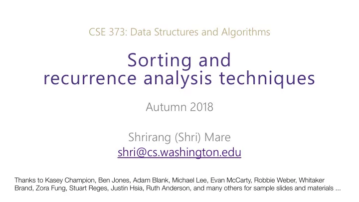
SLIDE 21

Tree Method Practice

21

!n# ! n 4

#

… … ! n 4

#

! n 4

#

! n 16

#

! n 16

#

! n 16

#

! n 16

#

! n 16

#

! n 16

#

! n 16

#

! n 16

#

! n 16

#

… … … … … … … … … … … … … … … … … … … … … … … … … 4 4 4 4 4 4 4 4 4 4 4 4 4 4 4 4 4 4 4 4 4 4 4 4 4 4 4 ' ( = 4 *ℎ,( ( ≤ 1 3' ( 4 + !(# 01ℎ,2*34,

EXAMPLE PROVIDED BY CS 161 – JESSICA SU HTTPS://WEB.STANFORD.EDU/CLASS/ARCHIVE/CS/CS161/CS161.1168/LECTURE3.PDF

' ( 4 ' ( 4 ' ( 4 ' ( 4 + ' ( 4 + ' ( 4 + !(#

Level (i) Number of Nodes Work per Node Work per Level 1 !(2 !(2 1 3 ! ( 4

#

3 16 !(# 2 9 ! ( 16

#

9 256 !(# 3 38 ! ( 48

#

3 16

8

!(# base 39:;<= 4 4 > 39:;<=

Combining it all together… ' ( = 4 (9:;<? + @

8AB 9:;C = DE

3 16

8

!(# Last recursive level: log< ( − 1

slide-22
SLIDE 22

Technique 3: Master Theorem

22

! " = $ %ℎ'" " = 1 )! " * + ",

  • .ℎ'/%01'

Given a recurrence of the following form: Where ), *, and 2 are constants, then !(") has the following asymptotic bounds ! " ∈ Θ ", log: ) < 2 log: ) = 2 ! " ∈ Θ ", log< " log: ) > 2 ! " ∈ Θ ">?@A B If If If then then then

slide-23
SLIDE 23

Apply Master Theorem

23

! " = 1 %ℎ'" " ≤ 1 2! " 2 + " +,ℎ'-%./'

! " = 0 %ℎ'" " = 1 1! " 2 + "3 +,ℎ'-%./' log7 1 = 8

! " ∈ Θ "3 log; "

log7 1 > 8 ! " ∈ Θ "=>?@ A If If ! " ∈ Θ "3 log7 1 < 8 If then then then

Given a recurrence of the form:

a = 2 b = 2 c = 1 d = 1

log7 1 = 8 ⇒ log; 2 = 1 ! " ∈ Θ "3 log; " ⇒ Θ "D log; "

slide-24
SLIDE 24

Reflecting on Master Theorem

The case

  • Recursive case conquers work more quickly than it divides work
  • Most work happens near “top” of tree
  • Non recursive work in recursive case dominates growth, nc term

The case

  • Work is equally distributed across call stack (throughout the “tree”)
  • Overall work is approximately work at top level x height

The case

  • Recursive case divides work faster than it conquers work
  • Most work happens near “bottom” of tree
  • Leaf work dominates branch work

24

! " = $ %ℎ'" " = 1 )! " * + ", -.ℎ'/%01' log5 ) = 6

! " ∈ Θ ", log9 "

log5 ) > 6 ! " ∈ Θ ";<=> ? If If ! " ∈ Θ ", log5 ) < 6 If then then then

Given a recurrence of the form:

log5 ) < 6 log5 ) = 6 log5 ) > 6

A')BC-/D ≈ $ ";<=> ? ℎ'0Fℎ. ≈ log5 ) */)"6ℎC-/D ≈ ",log5 )

slide-25
SLIDE 25
  • 1. Unfolding method
  • more of a brute force method
  • Tedious but works
  • 2. Tree methods
  • more scratch work but less error prone
  • 3. Master theorem
  • quick, but applicable only to certain type of recurrences
  • does not give a closed form (gives big-Theta)

Recurrence analysis techniques

CSE 373 AU 18 – SHRI MARE 25