Slaters condition: proof p* = inf x f(x) s.t. Ax = b, g(x) 0 - - PowerPoint PPT Presentation

slater s condition proof
SMART_READER_LITE
LIVE PREVIEW

Slaters condition: proof p* = inf x f(x) s.t. Ax = b, g(x) 0 - - PowerPoint PPT Presentation

Slaters condition: proof p* = inf x f(x) s.t. Ax = b, g(x) 0 e.g., inf x 2 s.t. e x+2 3 0 A = e.g., A = Picture of set A L(y,z) = Nonconvex example Interpretations L(x, y, z) = f(x) + y T (Axb) + z T g(x)


slide-1
SLIDE 1

Slater’s condition: proof

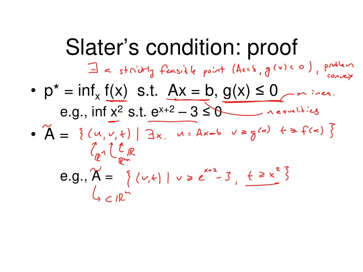
  • p* = infx f(x) s.t. Ax = b, g(x) ≤ 0

e.g., inf x2 s.t. ex+2 – 3 ≤ 0

  • A =

e.g., A =

slide-2
SLIDE 2

Picture of set A

L(y,z) =

slide-3
SLIDE 3

Nonconvex example

slide-4
SLIDE 4

Interpretations

L(x, y, z) = f(x) + yT(Ax–b) + zTg(x)

  • Prices or sensitivity analysis
  • Certificate of optimality
slide-5
SLIDE 5

Optimality conditions

  • L(x, y, z) = f(x) + yT(Ax–b) + zTg(x)
  • Suppose strong duality, (x, y, z) optimal
slide-6
SLIDE 6

Optimality conditions

  • L(x, y, z) = f(x) + yT(Ax–b) + zTg(x)
  • Suppose (x, y, z) satisfy KKT:

Ax = b g(x) ≤ 0 z ≥ 0 zTg(x) = 0 0 ∈ ∂f(x) + ATy + ∑i zi ∂gi(x)

slide-7
SLIDE 7

Using KKT

  • Can often use KKT to go from primal to

dual optimum (or vice versa)

  • E.g., in SVM:

αi > 0 <==> yi(xiTw + b) = 1

  • Means b = yi – xi

Tw for any such i

– typically, average a few in case of roundoff

slide-8
SLIDE 8

Set duality

  • Let C be a set with 0 ∈ conv(C)
  • C* = { y | xTy ≤ 1 for all x ∈ C }
  • Let K = { (x, s) | x ∈ sC }
  • K* = { (y, t) | xTy + st ≥ 0 for all X ∈ K }
slide-9
SLIDE 9

What is set duality good for?

  • Related to norm duality
  • Useful for helping visualize cones
slide-10
SLIDE 10

Duality of norms

  • Dual norm definition

||y||* = max

  • Motivation: Holder’s inequality

xTy ≤ ||x|| ||y||*

slide-11
SLIDE 11

Dual norm examples

slide-12
SLIDE 12

Dual norm examples

slide-13
SLIDE 13

Dual norm examples

slide-14
SLIDE 14

Cuboctahedron

slide-15
SLIDE 15

||y||* is a norm

  • ||y||* ≥ 0:
  • ||ky||* = |k| ||y||*:
  • ||y||* = 0 iff y = 0:
  • ||y1+y2||* ≤ ||y1||* + ||y2||*
slide-16
SLIDE 16

Dual-norm balls

  • { y | ||y||* ≤ 1 } =
  • Duality of norms:
slide-17
SLIDE 17

Visualizing cones

  • Suppose we have some weird cone in

high dimensions (say, K = S+)

  • Often easy to get a vector u in K ∩ K*

– e.g., I ∈ S+, I ∈ S+* = S+

  • Plot K ∩ { uTx = 1 } and K* ∩ { uTx = 1 }

instead of K, K*

– saves a dimension

slide-18
SLIDE 18

Visualizing S+

  • Say, 2 x 2 symmetric matrices
  • Add constraint tr(XTI) = 1
  • Result: a 2D set
slide-19
SLIDE 19
slide-20
SLIDE 20

What about 3 x 3?

  • 6 parameters in raw form
  • Still 5 after tr(X)=1
  • Try setting entire diagonal to 1/3

– plot off-diagonal elements

slide-21
SLIDE 21
slide-22
SLIDE 22

Visualizing 3*3 symmetric semidefinite matrices

slide-23
SLIDE 23

Multi-criterion optimization

  • Ordinary feasible region
  • Indecisive optimizer: wants all of
slide-24
SLIDE 24

Buying the perfect car

$K 0-60 MPG

slide-25
SLIDE 25

Pareto optimality

x* Pareto optimal =

slide-26
SLIDE 26

Pareto examples

slide-27
SLIDE 27

Scalarization

  • To find Pareto optima of convex problem: