Simulated Annealing Key idea: Vary temperature parameter, i.e. , - PDF document

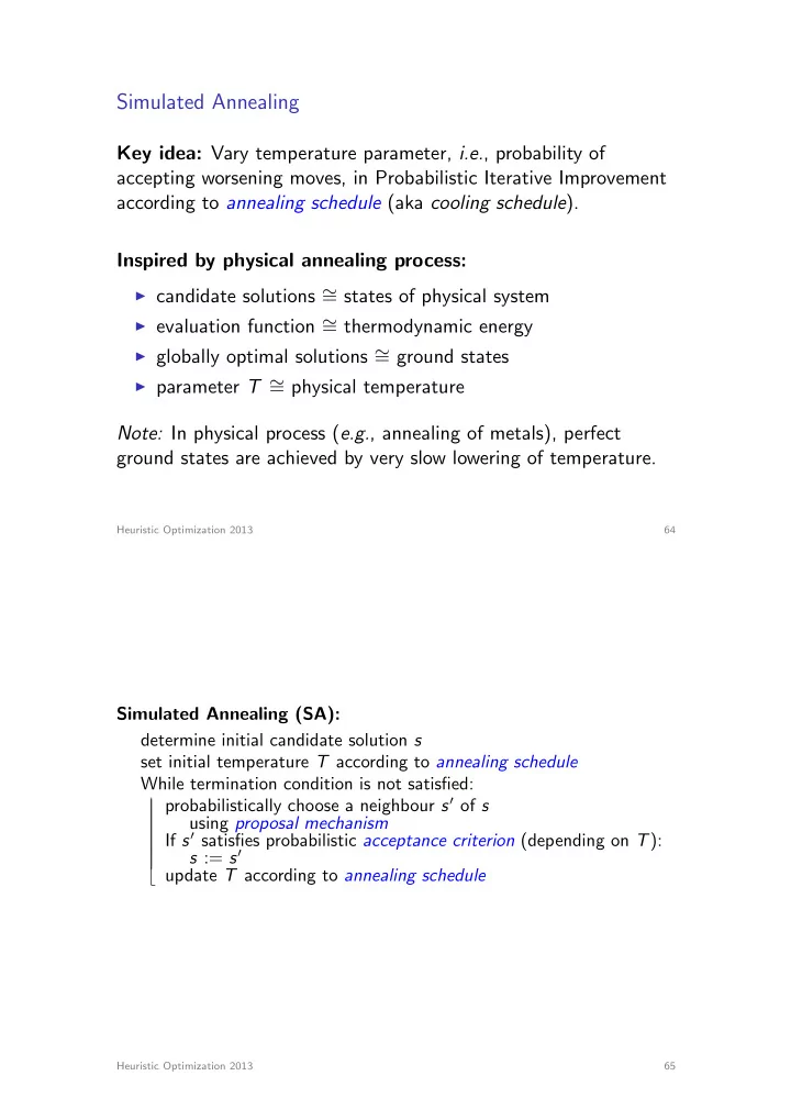
Simulated Annealing Key idea: Vary temperature parameter, i.e. , probability of accepting worsening moves, in Probabilistic Iterative Improvement according to annealing schedule (aka cooling schedule ). Inspired by physical annealing process: I candidate solutions ⇠ = states of physical system I evaluation function ⇠ = thermodynamic energy I globally optimal solutions ⇠ = ground states I parameter T ⇠ = physical temperature Note: In physical process ( e.g. , annealing of metals), perfect ground states are achieved by very slow lowering of temperature. Heuristic Optimization 2013 64 Simulated Annealing (SA): determine initial candidate solution s set initial temperature T according to annealing schedule While termination condition is not satisfied: | probabilistically choose a neighbour s 0 of s | | using proposal mechanism | | If s 0 satisfies probabilistic acceptance criterion (depending on T ): | | s := s 0 | b update T according to annealing schedule Heuristic Optimization 2013 65

Note: I 2-stage step function based on I proposal mechanism (often uniform random choice from N ( s )) I acceptance criterion (often Metropolis condition ) I Annealing schedule (function mapping run-time t onto temperature T ( t )): I initial temperature T 0 (may depend on properties of given problem instance) I temperature update scheme ( e.g. , geometric cooling: T := α · T ) I number of search steps to be performed at each temperature (often multiple of neighbourhood size) I Termination predicate: often based on acceptance ratio , i.e. , ratio of proposed vs accepted steps. Heuristic Optimization 2013 66 Example: Simulated Annealing for the TSP Extension of previous PII algorithm for the TSP, with I proposal mechanism: uniform random choice from 2-exchange neighbourhood; I acceptance criterion: Metropolis condition (always accept improving steps, accept worsening steps with probability exp [( f ( s ) � f ( s 0 )) / T ]); I annealing schedule : geometric cooling T := 0 . 95 · T with n · ( n � 1) steps at each temperature ( n = number of vertices in given graph), T 0 chosen such that 97% of proposed steps are accepted; I termination: when for five successive temperature values no improvement in solution quality and acceptance ratio < 2%. Heuristic Optimization 2013 67

Improvements: I neighbourhood pruning ( e.g. , candidate lists for TSP) I greedy initialisation ( e.g. , by using NNH for the TSP) I low temperature starts (to prevent good initial candidate solutions from being too easily destroyed by worsening steps) I look-up tables for acceptance probabilities: instead of computing exponential function exp( ∆ / T ) for each step with ∆ := f ( s ) � f ( s 0 ) (expensive!), use precomputed table for range of argument values ∆ / T . Heuristic Optimization 2013 68 Example: Simulated Annealing for the graph bipartitioning I for a given graph G := ( V , E ), find a partition of the nodes in two sets V 1 and V 2 such that | V 1 | = | V 2 | , V 1 [ V 2 = V , and that the number of edges with vertices in each of the two sets is minimal B A Heuristic Optimization 2013 69

SA example: graph bipartitioning Johnson et al. 1989 I tests were run on random graphs ( G n , p ) and random geometric graphs U n , d I modified cost function ( α : imbalance factor) f ( V 1 , V 2 ) = |{ ( u , v ) 2 E | u 2 V 1 ^ v 2 V 2 }| + α ( | V 1 | � | V 2 | ) 2 allows infeasible solutions but punishes the amount of infeasibility I side advantage : allows to use 1–exchange neighborhoods of size O ( n ) instead of the typical neighborhood that exchanges two nodes at a time and is of size O ( n 2 ) Heuristic Optimization 2013 70 SA example: graph bipartitioning Johnson et al. 1989 I initial solution is chosen randomly I standard geometric cooling schedule I experimental comparison to Kernighan–Lin heuristic I Simulated Annealing gave better performance on G n , p graphs I just the opposite is true for U n , d graphs I several further improvements were proposed and tested general remark: Although relatively old, Johnson et al.’s experimental investigations on SA are still worth a detailed reading! Heuristic Optimization 2013 71

‘Convergence’ result for SA: Under certain conditions (extremely slow cooling), any su ffi ciently long trajectory of SA is guaranteed to end in an optimal solution [Geman and Geman, 1984; Hajek, 1998]. Note: I Practical relevance for combinatorial problem solving is very limited (impractical nature of necessary conditions) I In combinatorial problem solving, ending in optimal solution is typically unimportant, but finding optimal solution during the search is (even if it is encountered only once)! Heuristic Optimization 2013 72 I SA is historically one of the first SLS methods (metaheuristics) I raised significant interest due to simplicity, good results, and theoretical properties I rather simple to implement I on standard benchmark problems (e.g. TSP, SAT) typically outperformed by more advanced methods (see following ones) I nevertheless, for some (messy) problems sometimes surprisingly e ff ective Heuristic Optimization 2013 73

Tabu Search Key idea: Use aspects of search history (memory) to escape from local minima. Simple Tabu Search: I Associate tabu attributes with candidate solutions or solution components. I Forbid steps to search positions recently visited by underlying iterative best improvement procedure based on tabu attributes. Heuristic Optimization 2013 74 Tabu Search (TS): determine initial candidate solution s While termination criterion is not satisfied: | determine set N 0 of non-tabu neighbours of s | | choose a best improving candidate solution s 0 in N 0 | | | | update tabu attributes based on s 0 | b s := s 0 Heuristic Optimization 2013 75

Note: I Non-tabu search positions in N ( s ) are called admissible neighbours of s . I After a search step, the current search position or the solution components just added/removed from it are declared tabu for a fixed number of subsequent search steps ( tabu tenure ). I Often, an additional aspiration criterion is used: this specifies conditions under which tabu status may be overridden ( e.g. , if considered step leads to improvement in incumbent solution). Heuristic Optimization 2013 76 Example: Tabu Search for SAT – GSAT/Tabu (1) I Search space: set of all truth assignments for propositional variables in given CNF formula F . I Solution set: models of F . I Use 1-flip neighbourhood relation , i.e. , two truth assignments are neighbours i ff they di ff er in the truth value assigned to one variable. I Memory: Associate tabu status (Boolean value) with each variable in F . Heuristic Optimization 2013 77

Example: Tabu Search for SAT – GSAT/Tabu (2) I Initialisation: random picking, i.e. , select uniformly at random from set of all truth assignments. I Search steps: I variables are tabu i ff they have been changed in the last tt steps; I neighbouring assignments are admissible i ff they can be reached by changing the value of a non-tabu variable or have fewer unsatisfied clauses than the best assignment seen so far ( aspiration criterion ); I choose uniformly at random admissible assignment with minimal number of unsatisfied clauses. I Termination: upon finding model of F or after given bound on number of search steps has been reached. Heuristic Optimization 2013 78 Note: I GSAT/Tabu used to be state of the art for SAT solving. I Crucial for e ffi cient implementation: I keep time complexity of search steps minimal by using special data structures, incremental updating and caching mechanism for evaluation function values; I e ffi cient determination of tabu status: store for each variable x the number of the search step when its value was last changed it x ; x is tabu i ff it � it x < tt , where it = current search step number. Heuristic Optimization 2013 79

Note: Performance of Tabu Search depends crucially on setting of tabu tenure tt : I tt too low ) search stagnates due to inability to escape from local minima; I tt too high ) search becomes ine ff ective due to overly restricted search path (admissible neighbourhoods too small) Advanced TS methods: I Robust Tabu Search [Taillard, 1991]: repeatedly choose tt from given interval; also: force specific steps that have not been made for a long time. I Reactive Tabu Search [Battiti and Tecchiolli, 1994]: dynamically adjust tt during search; also: use escape mechanism to overcome stagnation. Heuristic Optimization 2013 80 Further improvements can be achieved by using intermediate-term or long-term memory to achieve additional intensification or diversification . Examples: I Occasionally backtrack to elite candidate solutions , i.e. , high-quality search positions encountered earlier in the search; when doing this, all associated tabu attributes are cleared. I Freeze certain solution components and keep them fixed for long periods of the search. I Occasionally force rarely used solution components to be introduced into current candidate solution. I Extend evaluation function to capture frequency of use of candidate solutions or solution components. Heuristic Optimization 2013 81