outline
play

Outline Convergence DM812 METAHEURISTICS Lecture 2 1. Simulated - PowerPoint PPT Presentation

Simulated Annealing Outline Convergence DM812 METAHEURISTICS Lecture 2 1. Simulated Annealing Simulated Annealing 2. Convergence of Simulated Annealing Marco Chiarandini Department of Mathematics and Computer Science University of


  1. Simulated Annealing Outline Convergence DM812 METAHEURISTICS Lecture 2 1. Simulated Annealing Simulated Annealing 2. Convergence of Simulated Annealing Marco Chiarandini Department of Mathematics and Computer Science University of Southern Denmark, Odense, Denmark Simulated Annealing Simulated Annealing Outline Probabilistic Iterative Improv. Convergence Convergence Key idea: Accept worsening steps with probability that depends on respective deterioration in evaluation function value: bigger deterioration ∼ = smaller probability 1. Simulated Annealing Realization : Function p ( g, s ) : determines probability distribution over neighbors of s based on their values under evaluation function g . 2. Convergence of Simulated Annealing Let step ( s, s ′ ) := p ( f, s, s ′ ) . Note : Behavior of PII crucially depends on choice of p . II and RII are special cases of PII.
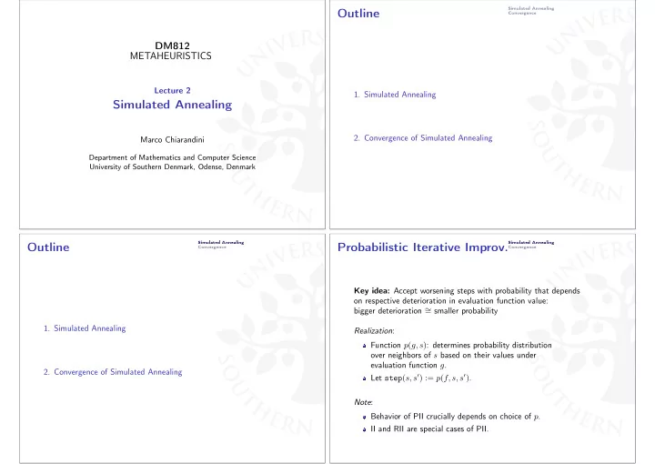
  2. Simulated Annealing Simulated Annealing Convergence Convergence Example: Metropolis PII for the TSP Search space S : set of all Hamiltonian cycles in given graph G . Solution set: same as S Inspired by statistical mechanics in matter physics: Neighborhood relation N ( s ) : 2-edge-exchange candidate solutions ∼ = states of physical system Initialization: an Hamiltonian cycle uniformly at random. evaluation function ∼ = thermodynamic energy Step function: implemented as 2-stage process: globally optimal solutions ∼ = ground states 1. select neighbor s ′ ∈ N ( s ) uniformly at random; parameter T ∼ = physical temperature 2. accept as new search position with probability: Note: In physical process ( e.g. , annealing of metals), perfect ground ( 1 if f ( s ′ ) ≤ f ( s ) states are achieved by very slow lowering of temperature. p ( T, s, s ′ ) := exp f ( s ) − f ( s ′ ) otherwise T (Metropolis condition), where temperature parameter T controls likelihood of accepting worsening steps. Termination: upon exceeding given bound on run-time. Simulated Annealing Simulated Annealing Simulated Annealing Convergence Convergence 2-stage step function based on proposal mechanism (often uniform random choice from N ( s ) ) Key idea: Vary temperature parameter, i.e. , probability of accepting acceptance criterion (often Metropolis condition ) worsening moves, in Probabilistic Iterative Improvement according to annealing schedule (aka cooling schedule ). Annealing schedule (function mapping run-time t onto temperature T ( t ) ): Simulated Annealing (SA): initial temperature T 0 determine initial candidate solution s (may depend on properties of given problem instance) set initial temperature T according to annealing schedule temperature update scheme while termination condition is not satisfied: do ( e.g. , linear cooling: T i +1 = T 0 (1 − i/I max ) , while maintain same temperature T according to annealing schedule geometric cooling: T i +1 = α · T i ) do number of search steps to be performed at each temperature probabilistically choose a neighbor s ′ of s using proposal (often multiple of neighborhood size) mechanism may be static or dynamic if s ′ satisfies probabilistic acceptance criterion (depending on T ) seek to balance moderate execution time with asymptotic behavior properties then s := s ′ Termination predicate: often based on acceptance ratio , update T according to annealing schedule i.e. , ratio of proposed vs accepted steps or number of idle iterations

  3. Simulated Annealing Convergence Example: Simulated Annealing for the TSP Extension of previous PII algorithm for the TSP, with proposal mechanism: uniform random choice from 2-exchange neighborhood; acceptance criterion: Metropolis condition (always accept improving steps, accept worsening steps with probability exp [( f ( s ) − f ( s ′ )) /T ] ); annealing schedule : geometric cooling T := 0 . 95 · T with n · ( n − 1) steps at each temperature ( n = number of vertices in given graph), T 0 chosen such that 97% of proposed steps are accepted; termination: when for five successive temperature values no improvement in solution quality and acceptance ratio < 2% . Improvements: neighborhood pruning ( e.g. , candidate lists for TSP) greedy initialization ( e.g. , by using NNH for the TSP) low temperature starts (to prevent good initial candidate solutions from being too easily destroyed by worsening steps) Simulated Annealing Simulated Annealing Profiling Related Approaches (1) Convergence Convergence Run A Run B 2.5 Noising Method Perturb the objective function by adding random noise. 2.0 The noise is gradually reduced to zero during algorithm’s run. Temperature 1.5 1.0 Threshold Method 0.5 Removes the probabilistic nature of the acceptance criterion 0.0 600 � 1 ∆( s, s ′ ) ≤ Q k p k (∆( s, s ′ )) = 500 0 otherwise Cost function value 400 Q k deterministic, non-increasing step function in k . 300 Suggested: Q k = Q 0 (1 − i/I MAX ) 200 100 0 0 10 20 30 40 50 0 10 20 30 40 50 Iterations 10 7 Iterations 10 7

  4. Simulated Annealing Simulated Annealing Related Approaches (2) Outline Convergence Convergence Critics to SA: The annealing schedule strongly depends on the time bound the search landscape and hence on the single instance Evidence that there are search landscapes for which optimal annealing 1. Simulated Annealing schedules are non-monotone [Hajek and Sasaki, Althofer and Koschnick, Hu, Kahng and Tsao]. Old Bachelor Acceptance Dwindling expectations 2. Convergence of Simulated Annealing � Q i + incr ( Q i ) if failed acceptance of s ′ Q i +1 = if s ′ accepted Q i − decr ( Q i ) decr ( Q i ) = incr ( Q i ) = T 0 /M a ) b − 1 � c ( age � � � i Q i = · ∆ · 1 − M ... (self-tuning, non-monotonic) Simulated Annealing Simulated Annealing Convergence Convergence ‘Convergence’ result for SA: ‘Convergence’ result for SA: Theorem ( [Geman and Geman, 1984; Hajek, 1998] ) Theorem ( [Geman and Geman, 1984; Hajek, 1998] ) Let � S, f, N � be the search landscape of a combinatorial optimization Let � S, f, N � be the search landscape of a combinatorial optimization problem with S ∗ � = S and S finite. Furthermore, let N be a problem with S ∗ � = S and S finite. Furthermore, let N be a neighborhood function defined on S that induces a strongly connected, neighborhood function defined on S that induces a strongly connected, symmetric neighborhood graph with diameter d . symmetric neighborhood graph with diameter d . Then the finite homogeneous Markov chain associated with a run of sim- If a cooling schedule is assumed in which the sequence { c k } ∞ k =1 of control ulated annealing at a fixed value c of the control parameter is strongly parameter values is non-increasing and satisfies both lim k →∞ = 0 and ergodic and the unique stationary distribution q ( c ) to which its probability c k ≥ d ∆ distribution converges satisfies log k c → 0 q i ( c ) = 0 lim with ∆ = max i ∈ S,j ∈ N ( i ) ( f ( j ) − f ( i )) , then the inhomogeneous Markov chain associated with a run of simulated annealing is strongly ergodic for any non-optimal solution i ∈ S . and the stochastic vector q to which its probability distribution converges satisfies q i = 0 for any non-optimal solution.

  5. Simulated Annealing Simulated Annealing Example Convergence Convergence Mathematical modelling of SA Note: Practical relevance for combinatorial problem solving is very limited (impractical nature of necessary conditions) In combinatorial problem solving, ending in optimal solution is typically unimportant, but finding optimal solution during the search is (even if it is encountered only once)! q (3) = (0 . 38 , 0 . 28 , 0 . 20 , 0 . 14) q (1) = (0 . 64 , 0 . 24 , 0 . 09 , 0 . 03) q (0 . 1) = (1 , 5 · 10 − 5 , 2 · 10 − 9 , 9 · 10 − 14 )

Download Presentation
Download Policy: The content available on the website is offered to you 'AS IS' for your personal information and use only. It cannot be commercialized, licensed, or distributed on other websites without prior consent from the author. To download a presentation, simply click this link. If you encounter any difficulties during the download process, it's possible that the publisher has removed the file from their server.

Recommend


More recommend