Shortest Cut Graph of a Surface with Prescribed Vertex Set ric - - PowerPoint PPT Presentation

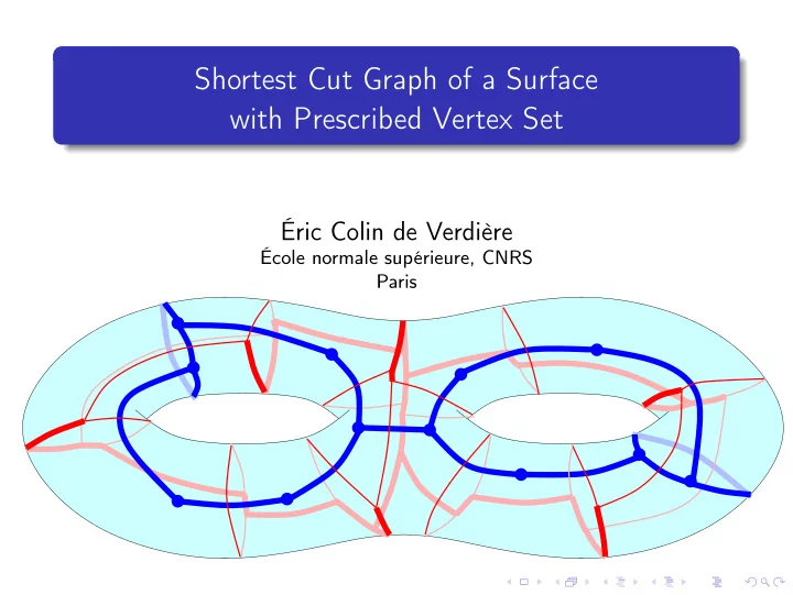
Shortest Cut Graph of a Surface with Prescribed Vertex Set

Éric Colin de Verdière

École normale supérieure, CNRS Paris

The Problem

Σ: compact surface without boundary; cut graph of Σ: graph embedded on Σ that cuts Σ into a topological disk. Goal: Given a finite point set P on Σ, compute the shortest cut graph with vertex set exactly P.

Why Cut a Surface into a Disk?

Applications Cutting a surface (into one or several planar pieces), to parameterize, put a texture, remesh, or compress it; sometimes, one needs to cut along lines of high curvature. The “length” function can be chosen arbitrarily, e.g., in relation to curvature.

[Favreau, Ph.D. thesis, 2009]

Why Cut a Surface into a Disk?

Applications Cutting a surface (into one or several planar pieces), to parameterize, put a texture, remesh, or compress it; sometimes, one needs to cut along lines of high curvature. The “length” function can be chosen arbitrarily, e.g., in relation to curvature. Theory Algorithms for nearly-planar graphs: separators, tree decompositions; building block for many algorithms to compute shortest graphs

• n surfaces:

shortest splitting cycle [Chambers et al., 2006], shortest curves within a given homotopy class [CdV and Erickson,

2006],

minimum cut [Chambers, Erickson, Nayyeri, 2009], shortest non-crossing walks [Erickson and Nayyeri, 2011], edgewidth and facewidth parameters [Cabello, CdV, Lazarus, 2010].

Comparison with Previous Work

Previous work

[Erickson and Har-Peled, 2004]:

computing the shortest cut graph (without fixing vertices) is NP-hard; O(log2 g)-approximation in small polynomial time.

[Erickson and Whittlesey, 2006]: fast algorithm to compute the

shortest cut graph with one single (given) vertex.

[CdV, 2003]: polynomial-time algorithm to compute the shortest

graph isotopic (with fixed vertices) to a given graph.

This talk

Generalization of the algorithm by [Erickson and Whittlesey] arbitrary finite set of vertices, possibly non-orientable surfaces. More natural proof The algorithm is greedy. (Most) optimal greedy algorithms fall within the matroid framework. I show that this is indeed the case here (via homology). Proof is therefore more natural and simpler.

Algorithm Description

Simultaneously grow a disk around each point in P. Compute the “Voronoi diagram” V of P, i.e., the set of points where these disks collide. A P-path is a path whose endpoints are in P. For each edge e of V, let δ(e) be the dual “Delaunay edge”: the shortest P-path crossing only edge e. Let the weight of e be the length of δ(e). Compute a maximum spanning tree T of V w.r.t. these weights. Return {δ(e) | e ∈ V \ T}.

Algorithm Description

Simultaneously grow a disk around each point in P. Compute the “Voronoi diagram” V of P, i.e., the set of points where these disks collide. A P-path is a path whose endpoints are in P. For each edge e of V, let δ(e) be the dual “Delaunay edge”: the shortest P-path crossing only edge e. Let the weight of e be the length of δ(e). Compute a maximum spanning tree T of V w.r.t. these weights. Return {δ(e) | e ∈ V \ T}.

Algorithm Description

Simultaneously grow a disk around each point in P. Compute the “Voronoi diagram” V of P, i.e., the set of points where these disks collide. A P-path is a path whose endpoints are in P. For each edge e of V, let δ(e) be the dual “Delaunay edge”: the shortest P-path crossing only edge e. Let the weight of e be the length of δ(e). Compute a maximum spanning tree T of V w.r.t. these weights. Return {δ(e) | e ∈ V \ T}.

Algorithm Description

Simultaneously grow a disk around each point in P. Compute the “Voronoi diagram” V of P, i.e., the set of points where these disks collide. A P-path is a path whose endpoints are in P. For each edge e of V, let δ(e) be the dual “Delaunay edge”: the shortest P-path crossing only edge e. Let the weight of e be the length of δ(e). Compute a maximum spanning tree T of V w.r.t. these weights. Return {δ(e) | e ∈ V \ T}.

Algorithm Description

Simultaneously grow a disk around each point in P. Compute the “Voronoi diagram” V of P, i.e., the set of points where these disks collide. A P-path is a path whose endpoints are in P. For each edge e of V, let δ(e) be the dual “Delaunay edge”: the shortest P-path crossing only edge e. Let the weight of e be the length of δ(e). Compute a maximum spanning tree T of V w.r.t. these weights. Return {δ(e) | e ∈ V \ T}.

Trivial Example: The Case of the Sphere

Problem reformulation Σ = Euclidean plane R2 with point at ∞ (sphere); We actually want to compute the minimum spanning tree of P. Well-known: MST(P) ⊆ Gab(P) ⊆ Del(P). What does the algorithm? computes a maximum spanning tree of the Voronoi diagram, where the weight of a Voronoi edge is the length of its dual “Delaunay” edge; the dual of the complement is the minimum spanning tree of the Delaunay triangulation, i.e., the minimum spanning tree of P.

Trivial Example: The Case of the Sphere

Problem reformulation Σ = Euclidean plane R2 with point at ∞ (sphere); We actually want to compute the minimum spanning tree of P. Well-known: MST(P) ⊆ Gab(P) ⊆ Del(P). What does the algorithm? computes a maximum spanning tree of the Voronoi diagram, where the weight of a Voronoi edge is the length of its dual “Delaunay” edge; the dual of the complement is the minimum spanning tree of the Delaunay triangulation, i.e., the minimum spanning tree of P.

Trivial Example: The Case of the Sphere

Problem reformulation Σ = Euclidean plane R2 with point at ∞ (sphere); We actually want to compute the minimum spanning tree of P. Well-known: MST(P) ⊆ Gab(P) ⊆ Del(P). What does the algorithm? computes a maximum spanning tree of the Voronoi diagram, where the weight of a Voronoi edge is the length of its dual “Delaunay” edge; the dual of the complement is the minimum spanning tree of the Delaunay triangulation, i.e., the minimum spanning tree of P.

Trivial Example: The Case of the Sphere

Problem reformulation Σ = Euclidean plane R2 with point at ∞ (sphere); We actually want to compute the minimum spanning tree of P. Well-known: MST(P) ⊆ Gab(P) ⊆ Del(P). What does the algorithm? computes a maximum spanning tree of the Voronoi diagram, where the weight of a Voronoi edge is the length of its dual “Delaunay” edge; the dual of the complement is the minimum spanning tree of the Delaunay triangulation, i.e., the minimum spanning tree of P.

Metric: Combinatorial Surfaces

A fixed weighted graph G on the surface gives the metric. The P-paths of the cut graph are restricted to lie in G and to be non-crossing. (All the δ(e) are non-crossing.)

Metric: Combinatorial Surfaces

A fixed weighted graph G on the surface gives the metric. The P-paths of the cut graph are restricted to lie in G and to be non-crossing. (All the δ(e) are non-crossing.)

Metric: Combinatorial Surfaces

A fixed weighted graph G on the surface gives the metric. The P-paths of the cut graph are restricted to lie in G and to be non-crossing. (All the δ(e) are non-crossing.)

Metric: Combinatorial Surfaces

A fixed weighted graph G on the surface gives the metric. The P-paths of the cut graph are restricted to lie in G and to be non-crossing. (All the δ(e) are non-crossing.)

Metric: Combinatorial Surfaces

A fixed weighted graph G on the surface gives the metric. The P-paths of the cut graph are restricted to lie in G and to be non-crossing. (All the δ(e) are non-crossing.)

Metric: Combinatorial Surfaces

A fixed weighted graph G on the surface gives the metric. The P-paths of the cut graph are restricted to lie in G and to be non-crossing. (All the δ(e) are non-crossing.) Running-time O(n log n) plus size of the output: O((g + |P|)n) where g is the genus of Σ and n is the complexity of G.

Greedy View of the Algorithm

begin end

Lemma Alternate way of computing the same result: iteratively add to a set S the shortest non-disconnecting Delaunay P-path p such that S ∪ {p} leaves Σ connected. To compute a maximum spanning tree of V: iteratively remove minimum-weight non-disconnecting edges in V. Each time we remove an edge e to V, we add the dual Delaunay edge δ(e) to a set S. Σ \ S is connected ⇔ V is connected.

Greedy View of the Algorithm

begin end

Lemma Alternate way of computing the same result: iteratively add to a set S the shortest non-disconnecting Delaunay P-path p such that S ∪ {p} leaves Σ connected. To compute a maximum spanning tree of V: iteratively remove minimum-weight non-disconnecting edges in V. Each time we remove an edge e to V, we add the dual Delaunay edge δ(e) to a set S. Σ \ S is connected ⇔ V is connected.

Greedy View of the Algorithm

begin end

Lemma Alternate way of computing the same result: iteratively add to a set S the shortest non-disconnecting Delaunay P-path p such that S ∪ {p} leaves Σ connected. To compute a maximum spanning tree of V: iteratively remove minimum-weight non-disconnecting edges in V. Each time we remove an edge e to V, we add the dual Delaunay edge δ(e) to a set S. Σ \ S is connected ⇔ V is connected.

Greedy View of the Algorithm

begin end

Lemma Alternate way of computing the same result: iteratively add to a set S the shortest non-disconnecting Delaunay P-path p such that S ∪ {p} leaves Σ connected. To compute a maximum spanning tree of V: iteratively remove minimum-weight non-disconnecting edges in V. Each time we remove an edge e to V, we add the dual Delaunay edge δ(e) to a set S. Σ \ S is connected ⇔ V is connected.

Greedy View of the Algorithm

begin end

Lemma Alternate way of computing the same result: iteratively add to a set S the shortest non-disconnecting Delaunay P-path p such that S ∪ {p} leaves Σ connected. To compute a maximum spanning tree of V: iteratively remove minimum-weight non-disconnecting edges in V. Each time we remove an edge e to V, we add the dual Delaunay edge δ(e) to a set S. Σ \ S is connected ⇔ V is connected.

Greedy View of the Algorithm

begin end

Lemma Alternate way of computing the same result: iteratively add to a set S the shortest non-disconnecting Delaunay P-path p such that S ∪ {p} leaves Σ connected. To compute a maximum spanning tree of V: iteratively remove minimum-weight non-disconnecting edges in V. Each time we remove an edge e to V, we add the dual Delaunay edge δ(e) to a set S. Σ \ S is connected ⇔ V is connected.

Greedy View of the Algorithm

begin end

Lemma Alternate way of computing the same result: iteratively add to a set S the shortest non-disconnecting Delaunay P-path p such that S ∪ {p} leaves Σ connected. To compute a maximum spanning tree of V: iteratively remove minimum-weight non-disconnecting edges in V. Each time we remove an edge e to V, we add the dual Delaunay edge δ(e) to a set S. Σ \ S is connected ⇔ V is connected.

Greedy View of the Algorithm

begin end

Lemma Alternate way of computing the same result: iteratively add to a set S the shortest non-disconnecting Delaunay P-path p such that S ∪ {p} leaves Σ connected. To compute a maximum spanning tree of V: iteratively remove minimum-weight non-disconnecting edges in V. Each time we remove an edge e to V, we add the dual Delaunay edge δ(e) to a set S. Σ \ S is connected ⇔ V is connected.

Greedy View of the Algorithm

begin end

Lemma Alternate way of computing the same result: iteratively add to a set S the shortest non-disconnecting Delaunay P-path p such that S ∪ {p} leaves Σ connected. To compute a maximum spanning tree of V: iteratively remove minimum-weight non-disconnecting edges in V. Each time we remove an edge e to V, we add the dual Delaunay edge δ(e) to a set S. Σ \ S is connected ⇔ V is connected.

Greedy View of the Algorithm

begin end

Lemma Alternate way of computing the same result: iteratively add to a set S the shortest non-disconnecting Delaunay P-path p such that S ∪ {p} leaves Σ connected. To compute a maximum spanning tree of V: iteratively remove minimum-weight non-disconnecting edges in V. Each time we remove an edge e to V, we add the dual Delaunay edge δ(e) to a set S. Σ \ S is connected ⇔ V is connected.

Greedy View of the Algorithm

begin end

Lemma Alternate way of computing the same result: iteratively add to a set S the shortest non-disconnecting Delaunay P-path p such that S ∪ {p} leaves Σ connected. To compute a maximum spanning tree of V: iteratively remove minimum-weight non-disconnecting edges in V. Each time we remove an edge e to V, we add the dual Delaunay edge δ(e) to a set S. Σ \ S is connected ⇔ V is connected.

Greedy View of the Algorithm

begin end

Lemma Alternate way of computing the same result: iteratively add to a set S the shortest non-disconnecting Delaunay P-path p such that S ∪ {p} leaves Σ connected. To compute a maximum spanning tree of V: iteratively remove minimum-weight non-disconnecting edges in V. Each time we remove an edge e to V, we add the dual Delaunay edge δ(e) to a set S. Σ \ S is connected ⇔ V is connected.

Greedy View of the Algorithm

begin end

Lemma Alternate way of computing the same result: iteratively add to a set S the shortest non-disconnecting Delaunay P-path p such that S ∪ {p} leaves Σ connected. To compute a maximum spanning tree of V: iteratively remove minimum-weight non-disconnecting edges in V. Each time we remove an edge e to V, we add the dual Delaunay edge δ(e) to a set S. Σ \ S is connected ⇔ V is connected.

Greedy View of the Algorithm

begin end

Lemma Alternate way of computing the same result: iteratively add to a set S the shortest non-disconnecting Delaunay P-path p such that S ∪ {p} leaves Σ connected. To compute a maximum spanning tree of V: iteratively remove minimum-weight non-disconnecting edges in V. Each time we remove an edge e to V, we add the dual Delaunay edge δ(e) to a set S. Σ \ S is connected ⇔ V is connected.

Greedy View of the Algorithm

begin end

Lemma Alternate way of computing the same result: iteratively add to a set S the shortest non-disconnecting Delaunay P-path p such that S ∪ {p} leaves Σ connected. To compute a maximum spanning tree of V: iteratively remove minimum-weight non-disconnecting edges in V. Each time we remove an edge e to V, we add the dual Delaunay edge δ(e) to a set S. Σ \ S is connected ⇔ V is connected.

Greedy View of the Algorithm

begin end

Lemma Alternate way of computing the same result: iteratively add to a set S the shortest non-disconnecting Delaunay P-path p such that S ∪ {p} leaves Σ connected. To compute a maximum spanning tree of V: iteratively remove minimum-weight non-disconnecting edges in V. Each time we remove an edge e to V, we add the dual Delaunay edge δ(e) to a set S. Σ \ S is connected ⇔ V is connected.

Preliminaries on Matroids and Greedy Algorithms

Minimum-weight basis of a vector space Let V be a vector space; let w : V → Z+ be a weight function. The greedy algorithm computes a minimum-weight basis of V : start with A = ∅; whenever possible, iteratively add to A a minimum-weight element linearly independent with A.

Preliminaries on Matroids and Greedy Algorithms

Minimum-weight basis of a vector space Let V be a vector space; let w : V → Z+ be a weight function. The greedy algorithm computes a minimum-weight basis of V : start with A = ∅; whenever possible, iteratively add to A a minimum-weight element linearly independent with A. Proof Greedy basis G = {g1, . . . , gk} in increasing order of weight,

• ptimal basis O = {o1, . . . , ok} in increasing order of weight.

If w(O) < w(G), then w(oi) < w(gi) for some i: G = { g1 ≤ g2 ≤ . . . ≤ gi−1 ≤ gi ≤ . . . ≤ gk } > O = { o1 ≤ o2 ≤ . . . ≤ oi−1 ≤ oi ≤ . . . ≤ ok }. At the ith step, one of {o1, . . . , oi} would be chosen instead of gi, contradiction!

Preliminaries on Matroids and Greedy Algorithms

Minimum-weight basis of a vector space Let V be a vector space; let w : V → Z+ be a weight function. The greedy algorithm computes a minimum-weight basis of V : start with A = ∅; whenever possible, iteratively add to A a minimum-weight element linearly independent with A. More generally. . . A matroid is a pair (V , I) where V is a set and I is a non-empty set

• f finite subsets of V such that:

if A ⊆ B ∈ I, then A ∈ I; if A, B ∈ I and |A| < |B|, then A ∪ {z} ∈ I for some z ∈ B \ A. Given w : V → Z+, the greedy algorithm finds a minimum-weight, inclusionwise maximal element of I.

Strategy of the Proof: the Hidden Matroid

Formally: 1-dimensional singular homology on surfaces, over Z/2Z, relatively to P. Rough sketch of proof (simplification)

1 We exhibit a matroid with base space the set of P-paths. 2 Let S be a set of non-crossing P-paths. Then S is an

independent set iff it does not disconnect Σ.

(In general, an independent set may contain crossing P-paths.)

3 Let S be an independent set, and p be the shortest P-path

such that S ∪ {p} is independent. Then p is Delaunay. This proves the result. . . The shortest maximal independent set can be computed greedily; the paths computed are Delaunay, and therefore non-crossing; thus the algorithm is identical to the previous one, and computes a shortest cut graph.

Strategy of the Proof: the Hidden Matroid

Formally: 1-dimensional singular homology on surfaces, over Z/2Z, relatively to P. Rough sketch of proof (simplification)

1 We exhibit a matroid with base space the set of P-paths. 2 Let S be a set of non-crossing P-paths. Then S is an

independent set iff it does not disconnect Σ.

(In general, an independent set may contain crossing P-paths.)

3 Let S be an independent set, and p be the shortest P-path

such that S ∪ {p} is independent. Then p is Delaunay. This proves the result. . . The shortest maximal independent set can be computed greedily; the paths computed are Delaunay, and therefore non-crossing; thus the algorithm is identical to the previous one, and computes a shortest cut graph.

Strategy of the Proof: the Hidden Matroid

Formally: 1-dimensional singular homology on surfaces, over Z/2Z, relatively to P. Rough sketch of proof (simplification)

1 We exhibit a matroid with base space the set of P-paths. 2 Let S be a set of non-crossing P-paths. Then S is an

independent set iff it does not disconnect Σ.

(In general, an independent set may contain crossing P-paths.)

3 Let S be an independent set, and p be the shortest P-path

such that S ∪ {p} is independent. Then p is Delaunay. This proves the result. . . The shortest maximal independent set can be computed greedily; the paths computed are Delaunay, and therefore non-crossing; thus the algorithm is identical to the previous one, and computes a shortest cut graph.

1 The Matroid

Z: Z/2Z-vector space of all sets of P-paths. B ⊆ Z: p1 + . . . + pk ∈ B iff there exist P-paths q1, . . . , qℓ such that the concatenation of the paths {p1, . . . , pk, q1, q1, q2, q2, . . . , qℓ, qℓ}, in some order, possibly after replacing some paths by their reversals, is a contractible cycle. B is a vector space included in Z. z1, . . . , zm ∈ Z are dependent if some non-trivial linear combination (sum) among the zi is in B. Z is a matroid!

1 The Matroid

Z: Z/2Z-vector space of all sets of P-paths. B ⊆ Z: p1 + . . . + pk ∈ B iff there exist P-paths q1, . . . , qℓ such that the concatenation of the paths {p1, . . . , pk, q1, q1, q2, q2, . . . , qℓ, qℓ}, in some order, possibly after replacing some paths by their reversals, is a contractible cycle. B is a vector space included in Z. z1, . . . , zm ∈ Z are dependent if some non-trivial linear combination (sum) among the zi is in B. Z is a matroid!

1 The Matroid

Z: Z/2Z-vector space of all sets of P-paths. B ⊆ Z: p1 + . . . + pk ∈ B iff there exist P-paths q1, . . . , qℓ such that the concatenation of the paths {p1, . . . , pk, q1, q1, q2, q2, . . . , qℓ, qℓ}, in some order, possibly after replacing some paths by their reversals, is a contractible cycle. B is a vector space included in Z. z1, . . . , zm ∈ Z are dependent if some non-trivial linear combination (sum) among the zi is in B. Z is a matroid!

1 The Matroid

Z: Z/2Z-vector space of all sets of P-paths. B ⊆ Z: p1 + . . . + pk ∈ B iff there exist P-paths q1, . . . , qℓ such that the concatenation of the paths {p1, . . . , pk, q1, q1, q2, q2, . . . , qℓ, qℓ}, in some order, possibly after replacing some paths by their reversals, is a contractible cycle. B is a vector space included in Z. z1, . . . , zm ∈ Z are dependent if some non-trivial linear combination (sum) among the zi is in B. Z is a matroid!

2 Independent = Non-Disconnecting

Lemma Let {p1, . . . , pk} be a set of non-crossing P-paths. Then {p1, . . . , pk} is an independent set iff it does not disconnect Σ. Proof of ⇒ by contraposition. Recall:

{z1, . . . , zm} ⊆ Z are dependent iff some non-trivial sum is in B. p1 + . . . + pk ∈ B iff there exist P-paths q1, . . . , qℓ such that the concatenation of the paths {p1, . . . , pk, q1, q1, q2, q2, . . . , qℓ, qℓ} in some order, possibly after replacing some paths by their reversals, is a contractible cycle.

2 Independent = Non-Disconnecting

Lemma Let {p1, . . . , pk} be a set of non-crossing P-paths. Then {p1, . . . , pk} is an independent set iff it does not disconnect Σ. Proof of ⇒ by contraposition. Recall:

{z1, . . . , zm} ⊆ Z are dependent iff some non-trivial sum is in B. p1 + . . . + pk ∈ B iff there exist P-paths q1, . . . , qℓ such that the concatenation of the paths {p1, . . . , pk, q1, q1, q2, q2, . . . , qℓ, qℓ} in some order, possibly after replacing some paths by their reversals, is a contractible cycle.

2 Independent = Non-Disconnecting

Lemma Let {p1, . . . , pk} be a set of non-crossing P-paths. Then {p1, . . . , pk} is an independent set iff it does not disconnect Σ. Proof of ⇒ by contraposition. Recall:

{z1, . . . , zm} ⊆ Z are dependent iff some non-trivial sum is in B. p1 + . . . + pk ∈ B iff there exist P-paths q1, . . . , qℓ such that the concatenation of the paths {p1, . . . , pk, q1, q1, q2, q2, . . . , qℓ, qℓ} in some order, possibly after replacing some paths by their reversals, is a contractible cycle.

3 Delaunay Property

Lemma Let S be an independent set, and z be the shortest set of P-paths such that S ∪ {z} is independent. Then z is a single Delaunay path. Proof: Linear algebra! Recall: T dependent ⇔ some non-trivial linear combination of elements in T is in the vector space B. Thus S ∪ {y} is independent ⇔ y is not a linear combination

• f elements in S and B.

Single path: Assume z = p1 + . . . + pk. Then for some i, S ∪ {pi} is independent. Since pi is no longer than z, we have z = pi. Single Delaunay path: Similar, using the fact that δ(ei) is the shortest path crossing ei:

Assume z crosses the edges e1, . . . , ek of V. Then z − (δ(e1) + . . . + δ(ek)) is in B. So for some i, S ∪ {δ(ei)} is

• independent. Since δ(ei) is no longer than z, we have z = δ(ei).

3 Delaunay Property

Lemma Let S be an independent set, and z be the shortest set of P-paths such that S ∪ {z} is independent. Then z is a single Delaunay path. Proof: Linear algebra! Recall: T dependent ⇔ some non-trivial linear combination of elements in T is in the vector space B. Thus S ∪ {y} is independent ⇔ y is not a linear combination

• f elements in S and B.

Single path: Assume z = p1 + . . . + pk. Then for some i, S ∪ {pi} is independent. Since pi is no longer than z, we have z = pi. Single Delaunay path: Similar, using the fact that δ(ei) is the shortest path crossing ei:

Assume z crosses the edges e1, . . . , ek of V. Then z − (δ(e1) + . . . + δ(ek)) is in B. So for some i, S ∪ {δ(ei)} is

• independent. Since δ(ei) is no longer than z, we have z = δ(ei).

3 Delaunay Property

Lemma Let S be an independent set, and z be the shortest set of P-paths such that S ∪ {z} is independent. Then z is a single Delaunay path. Proof: Linear algebra! Recall: T dependent ⇔ some non-trivial linear combination of elements in T is in the vector space B. Thus S ∪ {y} is independent ⇔ y is not a linear combination

• f elements in S and B.

Single path: Assume z = p1 + . . . + pk. Then for some i, S ∪ {pi} is independent. Since pi is no longer than z, we have z = pi. Single Delaunay path: Similar, using the fact that δ(ei) is the shortest path crossing ei:

Assume z crosses the edges e1, . . . , ek of V. Then z − (δ(e1) + . . . + δ(ek)) is in B. So for some i, S ∪ {δ(ei)} is

• independent. Since δ(ei) is no longer than z, we have z = δ(ei).

3 Delaunay Property

Lemma Let S be an independent set, and z be the shortest set of P-paths such that S ∪ {z} is independent. Then z is a single Delaunay path. Proof: Linear algebra! Recall: T dependent ⇔ some non-trivial linear combination of elements in T is in the vector space B. Thus S ∪ {y} is independent ⇔ y is not a linear combination

• f elements in S and B.

Single path: Assume z = p1 + . . . + pk. Then for some i, S ∪ {pi} is independent. Since pi is no longer than z, we have z = pi. Single Delaunay path: Similar, using the fact that δ(ei) is the shortest path crossing ei:

Assume z crosses the edges e1, . . . , ek of V. Then z − (δ(e1) + . . . + δ(ek)) is in B. So for some i, S ∪ {δ(ei)} is

• independent. Since δ(ei) is no longer than z, we have z = δ(ei).

Conclusion

Remark Every output P-path is: a shortest homotopic path, and the concatenation of two shortest paths plus an edge. Extensions This algorithm also solves the following problem: Given a surface with boundary, compute the shortest set of simple disjoint arcs that cut the surface into a disk. Extension to PL surfaces (non-crossing paths) and smooth (Riemannian) surfaces.

Conclusion

Remark Every output P-path is: a shortest homotopic path, and the concatenation of two shortest paths plus an edge. Extensions This algorithm also solves the following problem: Given a surface with boundary, compute the shortest set of simple disjoint arcs that cut the surface into a disk. Extension to PL surfaces (non-crossing paths) and smooth (Riemannian) surfaces. Naïve question (or open problem???) How to compute the shortest (=minimum-weight) triangulation of a surface with given vertex set? This is NP-hard in the Euclidean plane [Mulzer, Rote, 2006]; how hard is it in the combinatorial surface model?