Short-range radionuclide dispersion and deposition modelling EMRAS-2 - - PDF document

Short-range radionuclide dispersion and deposition modelling EMRAS-2 University of Seville model Introduction The model applied in the University of Seville has been specifically designed and developed for this scenario and for research purposes. It is a dynamic, process-oriented numerical model which simulates the dispersion of liquid and gas particles released after an explosion based upon a Lagrangian approach. The activity released by the explosion is considered to be in two forms: liquid and gas

• particles. A total amount of 10000 particles are released (5000 liquid and 5000 gas particles). Each

particle contains a certain amount of activity, depending on the 99m-Tc activity used in the experiment and on its fractionation among liquid and gas. Different dispersion processes are considered for liquid and gas, but in both cases the trajectories followed by individual particles are calculated until deposition, decay or until they leave the model domain. The model does not try to reproduce the explosion itself, but dispersion just after it. Thus, initial conditions for liquid particles consist of assuming an initial velocity for them, which is set as a calibration parameter. Liquid particles are released from the explosion container with such

• velocity. In the case of gas particles, a cloud above the explosion site is considered to be formed at a

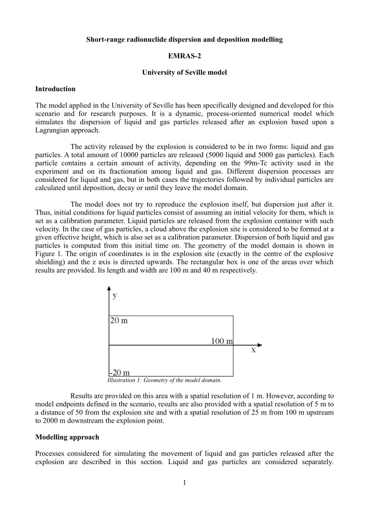
given effective height, which is also set as a calibration parameter. Dispersion of both liquid and gas particles is computed from this initial time on. The geometry of the model domain is shown in Figure 1. The origin of coordinates is in the explosion site (exactly in the centre of the explosive shielding) and the z axis is directed upwards. The rectangular box is one of the areas over which results are provided. Its length and width are 100 m and 40 m respectively. Results are provided on this area with a spatial resolution of 1 m. However, according to model endpoints defined in the scenario, results are also provided with a spatial resolution of 5 m to a distance of 50 from the explosion site and with a spatial resolution of 25 m from 100 m upstream to 2000 m downstream the explosion point. Modelling approach Processes considered for simulating the movement of liquid and gas particles released after the explosion are described in this section. Liquid and gas particles are considered separately. 1

Illustration 1: Geometry of the model domain.

Differences are due to a) different initial conditions for liquid and gas particles b) different dispersion mechanisms. Given the Lagrangian nature of the model, space is treated as a continuous, i.e., no spatial discretization is required. Model results can be provided over any resolution grid and there is not any limitation in this sense. A temporal discretization is required. Time step is provided as input data and typically is of the order of 10-2 seconds. Liquid particles Liquid particles are considered to follow a parabolic motion including friction with air. This friction is formulated in terms of a quadratic law with particle velocity. The friction coefficient is provided as input data. Additionally, particles are advected with wind velocity. Wind velocity and direction is provided in the scenario description and is assumed to be uniform over the model domain, although varying in time. Particles which touch the ground (z coordinate less or equal than zero) are deposited and do not move any more. Calculation stops for such particles. Radioactive decay is simulated using a Monte Carlo method. Calculation also stops for decayed particles. The explosive is initially confined by a box which is opened in the top and in one side. This shielding is considered to limit the direction of the initial velocity of liquid particles, both horizontally and vertically. Thus, in the horizontal, particles are initially confined by the angle - and +. In the vertical, particles are released between angles 1 and 2. These angles may be seen in Figure 2. Actual direction of the initial velocity of each liquid particles is obtained applying a Monte Carlo method, having all permitted directions the same probability. All angles are provided as input data. The magnitude of the initial velocity and a given error or tolerance (in %) for this parameter are also specified as input data through model calibration. The actual initial velocity magnitude for each particle is again obtained from a Monte Carlo method. However, velocity magnitude is assumed to obey a normal probability distribution with the specified mean value and standard deviation. 2

Gas particles Gas particles are considered to form a cloud over the explosion site. The dimension of this plume is defined in the scenario description: 7712 m3. Horizontally, the plume is centred over the explosion time. Vertically, it is centred about an effective release height provided as input data to the model. This effective height has been obtained after a calibration process. The particles are, initially, homogeneously distributed within this cloud. Again, the actual position of each gas particle within the cloud is obtained through a Monte Carlo method. Once initial positions of gas particles are obtained, these particles are advected by wind

• velocity. Three dimensional turbulent diffusion is calculated using a Monte Carlo method. The

diffusion coefficient is specified as input data. Particles which touch the ground are deposited and do not move any more. Radioactive decay is calculated using again a stochastic method. In order to calculate deposition, dose and air time-integrated activities over the grids defined in the scenario description, the spatial density of particles (liquid and gas) is calculated for each specified grid. Model parameters The following parameters are required by the model: 3

Illustration 2: Vertical (up) and horizontal (down) projection

• f the initial velocity of a given liquid particle. The possible

direction is limited by the specified angles.

• Calibrated parameters:

Initial velocity (m/s) and tolerance (%) of this value for liquid particles just after the explosion Friction coefficient of liquid particles with air Effective mean release height of gas particles (m) Fraction of activity released as aerosol particles. Some information is provided in the scenario, but the actual values had to be calibrated

• Parameters deduced or directly obtained from the scenario description:

Horizontal dispersion angle α Vertical dispersion angles Wind velocity vector components (m/s) Explosive shielding dimensions (m×m) Total activity released Time from activity determination in explosive to explosion itself

• Standard values

Diffusion coefficient in air (m2/s). Actually, a standard value does not exists, but a reasonable value

• f 30 m2/s has been used

Radioactive decay constant for 99m-Tc Dose conversion factor

• Simulation input

Simulation time (s) Time step (s) Uncertainties No uncertainty assessments are carried out. Model output The model provides deposited activity on the ground with a spatial resolution of 1 m (on a 1×1 m grid), time integrated activity in air with the same resolution in the horizontal and as a function of height (1 m vertical resolution) up to 30 m and also dose rates in the same grid as deposited activity. Model output has been arranged to provide results requested in the scenario description. Thus, the following files are provided:

• percentiles.out.- 95, 75 and 50 percentiles are provided in terms of the radius of a circle

containing the corresponding percentage of activity released by the explosion.

• surface_dose5.out.- surface contamination (Bq/m2) and dose rate (nGy/h) on a 5×5 m grid.

The first two columns of the file are the coordinates of the centre of the grid cell (y and x), the third column is surface contamination and the last one is dose rate.

• surface_dose25.out.- surface contamination (Bq/m2) and dose rate (nGy/h) on a 25×25 m
• grid. The first two columns of the file are the coordinates of the centre of the grid cell (y and

x), the third column is surface contamination and the last one is dose rate.

• centerline.out.- time integrated air concentrations (Bq×min/m3) as a function of the distance

to the explosion in m (first column) and averaged over 5 m length intervals. The other 5 columns give such concentrations at heights from 1 to 5 m over the ground. 4

Model application to the scenario The dose rate is calculated using a conversion factor given by the USEPA (Federal Guidance Report 12, EPA-402-R-93-081, External Exposure to Radionuclides in Air, Water and Soil), which gives the effective dose from the ground surface concentration of the radionuclide of interest. Tests 1 and 2 are used to calibrate the model. Once model parameters have been defined for these tests, the same values are used for tests 3 and 4 (except activity and time from activity measurement to explosion, obviously). Input data files for tests 1 and 2 are reproduced below:

input data for explosion code: test1

• 6.,40.

initial particle velocity (m/s), tolerance (%) 40. initial horizontal dispersion angle 30.,90. vertical angles 0.001 friction coefficient of liquid particles with air 30. diffusion coefficient in air (m^2/s) 16 simulated time (minutes) .01 time step (s) .80,.50 box explosive dimensions x,y (m) 780.e6 total activity (Bq) 3.20e-5 radioactive decay constant (s-1) 145. time in minutes from activity determination to explosion .35 fraction of activity in aerosol 25. effective mean release height for aerosol particles (m) input data for explosion code: test2

• 12.,40.

initial particle velocity (m/s), tolerance (%) 40. initial horizontal dispersion angle 30.,90. vertical angles 0.001 friction coefficient of liquid particles with air 30. diffusion coefficient in air (m^2/s) 16 simulated time (minutes) .01 time step (s) .80,.50 box explosive dimensions x,y (m) 1058.e6 total activity (Bq) 3.20e-5 radioactive decay constant (s-1) 80. time in minutes from activity determination to explosion .95 fraction of activity in aerosol 35. effective mean release height for aerosol particles (m)

For tests 2 to 4 most of the activity is thought to have been released as aerosol, thus, input data files for tests 3 and 4 are the same as for test 2 (except activity and time from its measurement to the explosion), since conditions are similar. Some examples of results are provided in the figures below. Vertical sections, along y- axis at several distances from the explosion site, of time integrated air concentrations are provided in Figure 3 in the case of test 2. 5

6

Illustration 3: Time integrated air concentrations. Vertical sections at different distances from the explosion site in logarithmic scale.

Horizontal maps of time integrated air concentrations at several heights above the ground, for test 2, are shown in Figure 4. For this experiment most of the activity (95%) is released as aerosol at an effective height of 35 m, thus it is not surprising that time integrated concentrations increase with increasing distance to the ground, both in Figures 3 and 4. Running time of the model is about 1 minute for a 16 minutes simulation on a PC compatible computer. The code is written in FORTRAN. In what follows, contour maps over the 5 and 25 m spatial resolution grids are provided. These maps are created with Matlab using the enclosed output files. Since the dose is directly proportional to the deposited activity, dose maps over the 25 m grid are not provided. Test 1 7

Illustration 4: Time integrated air concentrations, in logarithmic scale, at several heights above the ground.

8

Test 2 9

Test 3 10

11

Test 4 12

13