Selection of Linking Items Subset of items that maximally reflect - - PowerPoint PPT Presentation

Selection of Linking Items

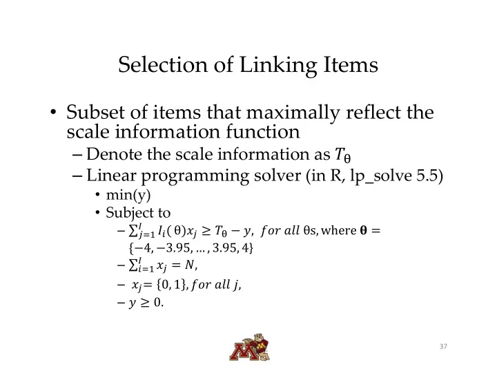
• Subset of items that maximally reflect the

scale information function

– Denote the scale information as – Linear programming solver (in R, lp_solve 5.5)

• min(y)
• Subject to

– ∑

• θ , θs, where

4, 3.95, … , 3.95, 4} – ∑

• ,

– 0, 1 , , – 0.

37

An example: Subscale 2

• Sum of Information Functions for 6‐, 7‐, and 8‐Item

Linking Sets

38

An example: Subscale 3

39

Why Fisher information is useful?

• In multidimensional CAT

– The volume of the confidence ellipsoid around

is proportional to the determinant

• f
• (Anderson, 1984)

– Maximize the determinant of the Fisher information matrix (Segall, 1996, Wang & Chang, 2011). D‐optimal method –

• 40

Fisher information vs. confidence ellipse

41

θ 15 10  θ 0.067 0.1 Σ

(Wang, et al., 2013)

Fisher information vs. confidence ellipse

42

θ 50 25  θ 0.02 0.04 Σ

(Wang, et al., 2013)

Mini‐max mechanism

• – Assuming there are three dimensions, then,

, ,

det

• ,

det

• ,

det

• ,

2 det

• ,

⋯ This criterion tends to pick the items that minimize the variance of the estimator lagging behind most

43

Item bank Information

44

Domain/Content balancing

• Constraint weighted D‐optimal (Wang et al., 2017)

– Suppose for each domain, we have maximum and minimum number of items set in advance, {, }, k=1,..,D

–

# of items belong to domain k so far, and n is

the current test length, is the maximum test length –

indicates whether item j belongs to domain k

–

∏

• (Cheng, et al., 2009)

–

=

• , =
• 45

A simulation study

46

• Sample size N=2,000
• Multivariate normal, with mean of 0’s, and

covariance matrix Σ=

• Maximum a Posteriori (MAP) is used, and prior is

multivariate normal with mean of 0’s and

• Evaluation criterion: root mean squared error

(RMSE)

2 1 1 1 1

1 ˆ RMSE( )= ( )

N i i i

N   







Results: Domain‐level recovery

47

D‐optimal (‐) vs. Random selection (‐‐‐)

Results: Domain‐level recovery

48

D‐optimal (‐) vs. Constraint‐weighted D‐optimal (‐‐)

Results: Domain‐level recovery

49

D‐optimal (‐) vs. Constraint‐weighted D‐optimal (‐‐)

Reducing Test Length

50

51

(0, 0, 0) Test Length

θ Confidence Interval

52

(2, 2, 2) Test Length

θ Confidence Interval

Variable‐length CAT: Stopping rule

53

Start 300+ items

Stopping rule

54

Start 300+ items

When the measurement precision criterion is satisfied

(Dodd, Koch & De Ayala, 1993; Boyd, Dodd, & Choi, 2010)

Stopping rule

55

Start 300+ items

(a) Volume of the confidence ellipsoid (D‐rule) (b) Sum of S.E. per domain θ (c) Maximum axis of the confidence ellipsoid (d) Kullback‐Leibler divergence between to consecutive posteriors

(Wang et al., 2013)

Cumulated information growth

56

Test Length

Determinant of Fisher information matrix

Stopping rule

57

Start 300+ items

Stopping rule

58

Start 300+ items

Stopping rule

59

Start 300+ items

(Babcock & Weiss, 2012 Wang et al., 2017+)

When θ does not change much: theta‐convergence rule (T‐rule)

• 0.01

Why T‐rule is secondary?

• 2PL

–

• ∗
• ,

∗ is in the

interval of (

• )

60

(Chang & Ying, 2008)

Why T‐rule is secondary?

• 2PL

–

• ∗
• ,

∗ is in the

interval of (

• )

– It does not monotonically decrease when test length increases!

• Terminate test pre‐maturely

61

(Wang et al., 2017+)

Why T‐rule is secondary?

• 2PL

–

• ∗
• ,

∗ is in the

interval of (

• )

– Undermine test efficiency

• Usually, the SE(

)<.2 (Dodd, et al., 1993)  25

• If hypothetically 1, satisfying

<.01 then ∗ 50

62

(Wang et al., 2017+)

MGRM

• Simple structure

63

• ,
• ∗

,

• 0:
• ,
• ∈ 1, … ,

2 : 1 ,

• ,
• ,
• ,
• 1:

,

• ,
• , exp

,

(Wang et al., 2017+)

MGRM

• Simple structure

64

• ,
• ∗

,

• 0:
• ,
• ∈ 1, … ,

2 : 1 ,

• ,
• ,
• ,
• 1:

,

• ,
• , exp

,

.5

(Wang et al., 2017+)

MGRM

• Complex structure

– If item j measures the pth trait

65

• ∗
• ∗

(Wang et al., 2017+)

MGRM

• Complex structure

– If item j measures the pth trait

66

pth element of

• (Wang et al., 2017+)
• ∗
• ∗

The amount of information carried by item j

MGRM

• Complex structure

– If item j measures the pth trait

67

(Wang et al., 2017+)

• ∗
• ∗

MGRM

• Complex structure

– If item j measures the pth trait – If item j measures multiple traits

68

(Wang et al., 2017+)

• ∗
• ∗
• ∗
• ∗

Primary vs. Secondary stopping rules

69

Start 300+ items

(Babcock & Weiss, 2012 Wang et al., 2017+) Minimum test length

Primary vs. Secondary stopping rules

70

Start 300+ items

Minimum test length If D‐rule is satisfied? (Wang et al., 2017+)

Primary vs. Secondary stopping rules

71

Start 300+ items

Minimum test length If D‐rule is satisfied? If T‐rule is satisfied? Yes No (Wang et al., 2017+)

Primary vs. Secondary stopping rules

72

Start 300+ items

Minimum test length If D‐rule is satisfied? Yes No If T‐rule is satisfied? Yes No Continue (Wang et al., 2017+)

Primary vs. Secondary stopping rules

73

Start 300+ items

Minimum test length If D‐rule is satisfied? Yes No If T‐rule is satisfied? Yes No Continue Maximum test length (Wang et al., 2017+) 94.9% 28.5 5.1% 61.5

Stopping rule results

74

θ

SE

Applied Cognition Daily Activity Mobility

3D plot

75

Stopping rule Cont.

76

Test length Overall precision Primary stop

Mean SD Bias RMSE Determinant Actual Eventual

28.5 13.3 0.005 0.303 514.7 0.949 0.965 1.6%

Stopping rule Cont.

77

Test length Overall precision Primary stop

Mean SD Bias RMSE Determinant Actual Eventual

28.5 13.3 0.005 0.303 514.7 0.949 0.965 Test length Bias RMSE Stop End Stop End Stop End Mean SD N=31 58.7 15.3 72.2 15.5 0.162 0.136 0.430 0.391 N=71 64.5 13.0 120 0.207 0.204 0.592 0.525 1.6%

Outline

• Brief introduction to computerized adaptive

testing (CAT)

• Multidimensional CAT
• “Computerized Adaptive Testing to Direct

Delivery of Hospital‐Based Rehabilitation”

(NIH R01HD079439, 2015‐2020)

– Item bank calibration – Item selection – Stopping rules

• Ongoing projects

78

Project I: Classification

79

FIM score FIM Stage

High

7

Independent Low

6

Modified independent High

5

Supervision Low

4

Contact guard High

2 ‐ 3

Min ‐ Mod Assist Low

1

Max Assist

Dependent (Red)

Red Dependent

Assistance (Orange) Table 2. AM‐PAC Color‐Coded Stages Independent (Green) Supervision ‐ Contact Guard (Yellow)

Project I: Classification

• Multidimensional CAT + Post‐hoc classification

Or

• Multidimensional Classification CAT?

80

Project II: Incorporating response time

(Fan, Wang, et al., 2012; Wang, et al., 2013a, 2013b; Wang & Xu, 2015)

• Exploratory data analysis (analysis per batch first)

– Histogram of batch 1 response time of all person‐item combinations (SD= 21.28, Skew= 41.84). Red line stands for the 97.5% percentile (25.85).

81

Project II: Incorporating response time

(Fan, Wang, et al., 2012; Wang, et al., 2013a, 2013b; Wang & Xu, 2015)

• Exploratory data analysis (analysis per batch first)

– After cutting the upper 2.5% of data (SD= 4.27, Skew= 1.23)

82

Project II: Incorporating response time

(Fan, Wang, et al., 2012; Wang, et al., 2013a, 2013b; Wang & Xu, 2015)

• Exploratory data analysis (analysis per batch first)

– After log‐transformation

83

Project II: Incorporating response time

(Fan, Wang, et al., 2012; Wang, et al., 2013a, 2013b; Wang & Xu, 2015)

• A hierarchical response time model (van der Linden,

2007)

84

Population μ,, σ, Item Item Person θ Person τ Item φ, λ

Four different models—EM algorithm

• (1) According to Molenaar, et al. (2015), we can re‐

parameterize van der Linden (2007)’s joint model as

– MGRM (

• )

–

• (2) Including interviewers as covariates, and the

interviewer effects differ across items

–

• 85

Correlation between and

Four different models—EM algorithm

• (3) Including interviewers as covariates, and the

interviewer effects differ across items by a same proportion

–

• (4) Including interviewers as fixed covariates

–

• 86

87

Model 1 Model 2 Model 3 Model 4

Model comparison & Results

Equation # of Free Parameters AIC BIC Batch 1

1 736 133566 136755 2 1281 133174 138725 3 741 133316 136527 4 741 133409 136620

Batch 2

1 652 102468 105202 2 940 102049 105992 3 655 102235 104982 4 655 102339 105086

Batch 3

1 656 111384 114149 2 1040 110613 114996 3 660 111001 113783 4 660 111323 114105

Batch 4

1 648 108550 111290 2 1028 107733 112080 3 652 108174 110931 4 652 108364 111121

88

θ θ θ 0.613 θ 0.466 0.853 Model 3 results (batch 1)

• Estimates of are:

0.591, 0.691 and 0.596

• Compared to MGRM

alone, adding response time results in higher item discrimination parameter estimates and smaller standard errors.

Concurrent calibration across 4 batches

• Adding response time information did not

affect the item parameter estimates and their standard errors significantly;

• Adding response time information helped

reduce the standard error of patients’ multidimensional latent trait estimates, but adding interviewer as a covariate did not result in further improvement.

89

Next steps II: Incorporating response time

(Fan, Wang, et al., 2012; Wang, et al., 2013a, 2013b; Wang & Xu, 2015)

• A hierarchical response time model (van der Linden,

2007)

• Maximize item information per time unit

90

Maximize

• |

Next steps III: DIF‐CAT

(Wang, Weiss, & Wang, 2017)

• 3 factors to consider

– Gender (Male/Female) – Education (College+/high school and below) – Age (<65/65~90)

91

Example DIF items

• Gender

– How much difficulty do you currently have making decisions, such as what clothes you want to wear? (Applied Cognition), consistent with expert hypothesis.

• Age

– How much difficulty do you currently have removing a plastic lid from a hot beverage cup? (Daily activity) – How much difficulty do you currently have climbing stairs step‐over‐step without a handrail? (Mobility)

92

How to deal with DIF in a CAT design?

• Items with extreme DIF—delete?
• Items with small DIF—keep?
• “Doubly adaptive CAT using subgroup

information to improve measurement precision”

(Wang et al., 2017) – Allow DIF items to have different parameters per subgroup

• Constraint weighted D‐optimal

93

Project IV: Adaptive measure of change

(Wang & Weiss, 2017, Wang, 2014)

• Specifying the MCAT to efficiently detect meaningful

clinical change

94

Study I

95

Project IV: Adaptive measure of change

(Wang & Weiss, 2017, Wang, 2014)

96

Time 1 Time 2

θ

Project IV: Adaptive measure of change

(Wang & Weiss, 2017, Wang, 2014)

• Item selection?—Select an item that can best differentiate

null hypothesis (no individual change) from alternative hypothesis.

• Sequential hypothesis testing?‐‐‐Stopping rule

97

Time 1 Time 2

• 2

( 1)

ˆ ˆ ( , )

pooled i i L j k

KL  

 

maximize

θ

Algorithms Web‐based delivery Data collection with MCAT

98

Monitor item usage, and routinely recalibrate item parameters if needed

(Chen & Wang, 2016)

My collaborators and team

99

• Dr. David Weiss

University of Minnesota

• Dr. Andrea Cheville

Mayo Clinic

Research Assistants: Zhuoran Shang Shiyang Su