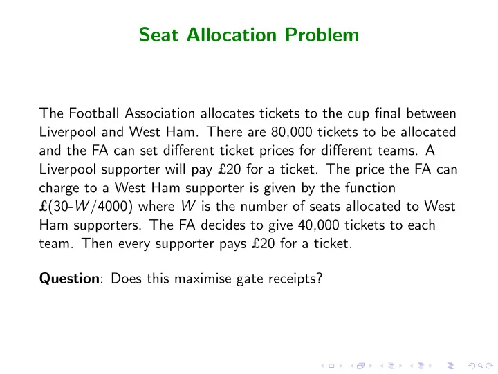
Seat Allocation Problem The Football Association allocates tickets - - PowerPoint PPT Presentation

Seat Allocation Problem

The Football Association allocates tickets to the cup final between Liverpool and West Ham. There are 80,000 tickets to be allocated and the FA can set different ticket prices for different teams. A Liverpool supporter will pay ↔20 for a ticket. The price the FA can charge to a West Ham supporter is given by the function

↔(30-W /4000) where W is the number of seats allocated to West

Ham supporters. The FA decides to give 40,000 tickets to each

• team. Then every supporter pays ↔20 for a ticket.

Question: Does this maximise gate receipts?

Nuts and Bolts

A nut and bolt factory has two divisions producing nuts and bolts. The income statement for sales and costs is given in the following table: Nuts Bolts Total Sales 225 225 450 Less: Variable Costs 150 190 340 Allocated Overhead 50 50 100 Net Contribution 25 (15) 10 Question: Since the Bolt division makes a loss should it be closed down?

Should Freedonia Export Steel?

Freedonia has a monopoly steel manufacturer which sells steel at

↔680 per ton, which is well above the world price of ↔375 per ton.

All imports of steel into Freedonia are barred. The firm does not export steel. Why should it? It would only get ↔375 by exporting a ton and can get ↔680 a ton by producing domestically. Moreover, the lowest average cost at which the firm can produce steel is ↔400 per ton. So it is argued that selling at ↔375 per ton is never profitable. Claim: Contrary to this argument, the firm might increase profits by exporting. Why?

The Tragedy of the Commons

A lake is used by the fishermen of the local village. There are 100 villagers who either fish or farm. If B boats fish, then the catch per boat is 80/ √

• B. The cost of running the boat is ↔3 and the

fishermen could alternatively work the land for a wage of ↔7. The price of fish is determined at the market in the town and is ↔1 no matter how many fish are caught. Fishermen will fish provided the profit they make by fishing exceeds what they can earn by working the land. Claim: There will be overfishing of the lake. 64 boats will fish when village income would be maximised by having 16 boats

• fishing. Why?

Poiuyt Example

A firm produces “poiuyts”. If it sells x poiuyts the price it will receive per poiuyt is P(x) = 6 − 3 5000x. The revenue it receives is x × P(x) so that TR(x) := xP(x) = 6x − 3 5000x2 The total cost of making x poiuyts is TC(x) = 1000 + x + x2 5000.

Excel Spreadsheet Chapter 3-1

Multivariate Optimisation

A butcher sells pork and beef, which are substitutes. The prices of pork and beef are Pp(xp, xb) = 90 − xp 100 − xb 300 Pb(xp, xb) = 120 − xb 100 − xp 150. The butcher’s total costs are TC(xp, xb) = 1000 + 10xp + 20xb. How should xp and xp be chosen to maximise profits?

Excel Spreadsheet Chapter 3-2

Freedonia Steel

Suppose that the price at which the Steel company can sell its steel domestically if it sells x units is P(x) = 1000 − x 250. Suppose the firm’s total cost function is TC(x) = 10, 000, 000 + 200x + x2 1000. Suppose y is the export sales of the firm at the fixed world price of

↔375. Question: Is y > 0?

Discrete Optimisation

◮ The Nut and Bolt example is one of discrete optimisation —

shut down or don’t shut down.

◮ It is nevertheless possible to use the logic of marginal analysis. ◮ A decision should be based on the marginal or incremental

impact of that decision on overall profits.

◮ In the example overhead costs were allocated equally across

divisions but different cost allocation rules (such as proportional sales) can give rise to the same contradictions. [See Exercise 3.7]

Global versus Local Optimisation

Constrained Optimisation

◮ Consider the ticket allocation problem. ◮ The problem is constraint because the total tickets allocated

cannot exceed 80,000.

◮ Turn a constrained optimisation problem into an

unconstrained one.

◮ Ask the marginal question: should seats be reallocated

between the two teams’ supporters on the margin.

◮ Check that the reallocation increases overall gate receipts.

Optimisation and Efficiency

◮ Consider the fishing problem. ◮ Acting individually each fisherman will fish provided fishing

yields more than farming. 80 √ B − 3 ≥ 7.

◮ Village income could be improved by choosing B to maximize

B 80 √ B − 3

• + 7(100 − B).

◮ There is overfishing because the individual fishermen do not

take into account the marginal impact they have of decreasing the catch of the other fishermen.

◮ Check that village income is increased. ◮ Could the optimal solution be implemented?

Summary

◮ Profit is maximised by equating marginal revenue to marginal

cost.

◮ Marginal revenue is not generally the price of the last unit

• sold. It is usually less than this.

◮ For discrete choices one cannot use calculus but the same

logic of marginal or incremental impact applies.

◮ Maximisation is more complicated in constrained optimisation

problems but it usually works to think of the marginal contributions of different activities (as in the ticket allocation problem)

◮ Individual maximisation is not the same as efficiency.

Double Marginalisation

Question: What is worse than a monopoly?

Double Marginalisation

Question: What is worse than a monopoly? Answer: A chain of monopolies.

Examples

◮ The ancient silk route

◮ Beginning around 200 B.C., there was a major trade of silk

from China to Rome involving five contiguous powers: the Roman empire, the Parthian empire, the Kushan empire, the nomadic confederation of the Xiongnu, and the Han empire

◮ ISP which sell internet access to consumers buy connections

from the phone companies, typically BT.

◮ Car manufacturers and retailers.

◮ the case of Porsche in the USA

◮ Manufacturer and retailer - distribution chain

What do we want to know?

Suppose there is a wholesaler/manufacturer M and a retailer R. Suppose the manufacturer sells to the retailer at price p and the retailer sells to customers at price P. If the retailers sells x units, the price it receives per unit is given by a function P(x). We want to know:

What do we want to know?

Suppose there is a wholesaler/manufacturer M and a retailer R. Suppose the manufacturer sells to the retailer at price p and the retailer sells to customers at price P. If the retailers sells x units, the price it receives per unit is given by a function P(x). We want to know:

◮ What price p should the manufacturer choose to maximise

profits? What price P should the retailer charge? What are the profits of the two firms?

What do we want to know?

Suppose there is a wholesaler/manufacturer M and a retailer R. Suppose the manufacturer sells to the retailer at price p and the retailer sells to customers at price P. If the retailers sells x units, the price it receives per unit is given by a function P(x). We want to know:

◮ What price p should the manufacturer choose to maximise

profits? What price P should the retailer charge? What are the profits of the two firms?

◮ If the manufacturer can market directly, should she? Will

customers prefer this?

What do we want to know?

Suppose there is a wholesaler/manufacturer M and a retailer R. Suppose the manufacturer sells to the retailer at price p and the retailer sells to customers at price P. If the retailers sells x units, the price it receives per unit is given by a function P(x). We want to know:

◮ What price p should the manufacturer choose to maximise

profits? What price P should the retailer charge? What are the profits of the two firms?

◮ If the manufacturer can market directly, should she? Will

customers prefer this?

◮ Is there anything else the manufacturer can do, other than

marketing directly, which can increase its profits?

An Example

Suppose the inverse demand function is P(x) = 131 −

x 100.

Suppose the manufacturer has a cost function TC(x) = 11x. Manufacturer profits are πM(x) = x(p − 11). Retailer profits are πR(x) = xP(x) − px = x

• 131 −

x 131

• − px.

The retailer will maximise profits by choosing x = 50(131 − p). Prove. The manufacture can choose price p to maximise πM(x) = 50(131 − p) (p − 11). The solution is p = 71. Therefore x = 3, 000, P = 101. Check. What are profits?

Excel Spreadsheet Porsche Chapter 6

The Double Marginalisation

3000 11 71 101 131

Price Quantity

Direct Selling

If the manufacturer can sell directly at no additional cost, then it will set a retail price P = 71, sell 6,000 units for profits of 360,000. Profits are increased and consumers pay lower prices and get more units. If the manufacturer incurs an additional marginal cost k to market directly, then it will set the retail price at P = 71 + k

• 2. Check.

Customers prefer the direct marketing if k < 60. Check. The manufacturer prefers it if k < 60(2 − √ 2) ≃ 35.15. Check.

Charging a Franchise Fee F

Suppose the manufacturer charges an upfront fee of F to the retailer for the right to sell her product. How big can F be? When the wholesale price is p, the retailer’s profit is 25(131 − p)2. If the manufacturer sets F = 25(131 − p)2, her profits are 25(131 − p)2 + 50(131 − p)(p − 11). which is maximised when p = 11. Check. The manufacturer’s total profit is 360,000, i.e. the profits it would get if it marketed directly and had a zero retailing cost!

The Single Marginalisation

6000 11 71 131

Price Quantity

Vertical Restraints

There are methods other than the fixed fee (two-part tariff) of achieving something similar:

◮ Resale price maintainence - setting a maximum or minimum

resale price.

◮ Quantity forcing

These types of vertical restraints that overcome the double marginalistion problem are as we have seen usually welfare enhancing.

Vertical Integration

◮ Another possibility is that the two firms could merge. Because

we have an upstream firm, a manufacturer, supplying to a downstream firm, in this case a retailer, such a merger is known as vertical integration.

◮ Expansion of activities downstream is referred to as forward

integration, and expansion upstream is referred to as backward integration.

◮ How much would the manufacturer pay to merge with the

retailer?

◮ Suppose the manufacturer has retailing costs of 30. ◮ It prefers to market directly and then sells at 86 for a profit of

202,500. Check.

◮ By owning the retailers and having its cost advantage in

marketing, it could increase profits to 360,000.

◮ Therefore it would pay up to 157,500 to acquire the retailer.

Are vertical restraints good or bad?

Some good reasons:

◮ Avoids double marginalisation ◮ Retailer service and free-riding

◮ Manufacturers investment in retailing can be protected by

exclusive dealerships to avoid retailer incentives to sell other more profitable lines.

◮ Minimum resale prices might lead retailers to compete on

quality rather than price thus avoiding a horizontal externality than good service in one outlet may benefit other outlets too.

◮ Minimum resale prices might generate retailer profits that

mean franchisees have something to lose if their contract is terminated.

◮ Exclusive territories might help avoid the hold-up problem for

the franchisee’s investment.

Are vertical restraints good or bad?

The same vertical constraints can also be anti-competitive.

◮ Production companies like HBO sell programmes to cable

• perators like Time Warner. Time Warner backward

integrates and buys HBO. It creates an incentive for Time Warner to favour HBO at the expense of rival programme

• producers. This is known as foreclosure.

◮ Exclusive territories can reduce competition and reduce

consumer surplus.

◮ Buying a supplier can raise the proportion of fixed costs and

thus help deter entry. Example: Amazon acquiring warehousing books rather than simply selling them. This can make them much more aggressive price competitors.

Summary

◮ There are costs to multiple-marginalisation. ◮ The costs can be overcome by a fixed fee (two-part tariff). ◮ This is welfare enhancing. Producer profit and consumer

surplus goes up.

◮ Sometimes the two-part tariff is refereed to as a vertical

restraint.

◮ Vertical constraints can sometimes be good and sometimes be

anti-competitive.

◮ The two-part tariff is also used as a method of price

discrimination which is our next topic.

Price Discrimination

◮ What is price discrimination?

Price Discrimination

◮ What is price discrimination?

◮ Charging high prices to customers who will pay high prices and

not charging high prices to those that won’t.

◮ Extracting as much surplus out of consumers from their

purchases.

Price Discrimination

◮ What is price discrimination?

◮ Charging high prices to customers who will pay high prices and

not charging high prices to those that won’t.

◮ Extracting as much surplus out of consumers from their

purchases.

◮ What are the difficulties in price discriminating?

Price Discrimination

◮ What is price discrimination?

◮ Charging high prices to customers who will pay high prices and

not charging high prices to those that won’t.

◮ Extracting as much surplus out of consumers from their

purchases.

◮ What are the difficulties in price discriminating?

◮ Knowing who is who. ◮ Keeping the deals intended for one group of consumers out of

the hands of another group they weren’t intended for.

◮ Knowing how rivals will react. ◮ Preventing customers bargaining back

Examples of Price Discrimination

◮ Airline pricing ◮ International pricing by pharmaceutical companies ◮ Soft and hard cover books ◮ Methyl Methacrylate ◮ Mobile phone contracts ◮ Armani ◮ IBM LaserPrinter E ◮ Coupons ◮ Student discounts ◮ Car parking on campus

Mr Inelastic and Mrs Elastic

Profit Maximisation Again

At the profit maximising point MR(x) = MC(x). Since TR(x) = xP(x), MR(x) = dTR(x) dx = x dP(x) dx + P(x) Therefore MR(x) = MC(x) implies x dP(x) dx + P(x) = MC(x) which can be rearranged as P(x) − MC(x) P(x) = − x P(x) dP(x) dx .

The Mark-Up Rule

On further rearrangement this gives P − MC P = 1 η where η = −P x dx dP is the elasticity of demand. The left-hand-side of the above equation is the mark-up. There are two things to note here:

◮ The LHS is less than one so η must be greater than one. ◮ the more inelastic is demand (smaller η) the greater is the

price.

Exercise

A monopolist sells in two different markets with demand curves given by P1(x1) = 10 − x1 and P2(x2) = 20 − x2. Total costs are TC(x1 + x2) = 5 + 2(x1 + x2). Calculate the profit maximising quantities and prices in the two markets. What is the elasticity of demand in each market. Hint: Calculate marginal revenue and marginal cost in each market.

A Taxonomy of Price Discrimination

Price discrimination is usually divided into three types which are uninspiringly call first-degree, second-degree and third-degree price discrimination.

◮ Third-degree or direct price discrimination.

◮ Charge different groups of customers different price based on

location, status, age, other purchases, time etc.

◮ Second-degree or indirect price discrimination.

◮ Customers are offered a non-linear price schedule and allowed

to choose how much to buy and what tariff to accept.

◮ First-degree or perfect price discrimination.

◮ There is a separate deal for nearly every customer.

Third-Degree or Direct Price Discrimination

◮ Firm sells same basic good in different forms or in with

different conditions attached to discriminate amongst groups

• f customers.

◮ This is our example of selling in two different locations. ◮ Demand is often interdependent (e.g. hard and soft cover

textbooks) and this makes situation slightly more complicated.

◮ Time can be used as a discriminator. ◮ Yield or revenue management schemes are very sophisticated

and rarely optimal.

◮ To succeed it is necessary to stop arbitrage between groups.

This is easiest if: transport costs are high; there are legal restrictions on resale; products or prices are personalised; markets are thin; there are informational problems.

Second-Degree or Indirect Price Discrimination

◮ Quantity discounts are one for of indirect price discrimination. ◮ Discounts could be for large or small purchases. ◮ In the first case this may be better for the firm than

discriminating by groups. In the second case it probably isn’t.

◮ Non-linear schemes can face implementation problems.

The Extraction of Surplus

◮ Second-degree price discrimination can improve profits even

when all customers are identical. If the consume has a utility function u(x) + m then the surplus a customer gets from a transaction is (u(x∗) + m0 − px∗) − (u(0) + m0) = u(x∗) − u(0) − px∗ ≥ 0. The customer will pay an up-front fee of F if u(x∗) − u(0) − px∗ > F.

◮ But can the firm know u(x) for each customer and could it

charge different fees for different customers?

Take-it-or-leave-it Offers

Suppose the firms say to the customer you must buy ˆ x for a total price of Q. Take it or leave it. The customer will accept if u(ˆ x) + m0 − Q ≥ u(0) − m0,

• r

u(ˆ x) − u(0) ≥ Q. Assume constant marginal costs of c and the firm sets Q as high as possible. Then firm profits are Q − cˆ x = u(ˆ x) − u(0) − cˆ x. The firm would optimally choose ˆ x where du(ˆ x)/dx = c.

Getting the Customer to Choose

Suppose that the firm sets p = c and F = u(ˆ x) − u(0) − cˆ x where ˆ x satisfies du(ˆ x)/dx = c. The customer, if he or she accepts the deal chooses x to maximise utility u(x) − u(0) − cx − F. So chooses x = ˆ

• x. The customer chooses of his/her own free will

the take-it-or-leave-it offer!

First-degree or Perfect Price Discrimination

◮ First-degree price discrimination would be setting a price equal

marginal cost and a fixed fee (different) for every customer.

◮ This might be illegal or unethical. ◮ It might be hard to prevent resale. ◮ Customers might start bargaining.

Summary

◮ Price discrimination can increase profits. ◮ Price discrimination is pervasive. ◮ There are different types of price discrimination, direct and

indirect.

◮ Aims of price discrimination are: (i) to get customers with

inelastic demands paying more and customers with elastic demands paying less; (ii) extracting more surplus from the customer.

◮ There are difficulties in preventing customers arbitraging

amongst themselves and bargaining back.

◮ Price discrimination schemes can be very complex and may be

difficult to design optimally.

Perfect Competition

◮ Examine interactions among firms. ◮ Focus on equilibrium in which actions are maximising given

what other firms or individuals do.

◮ Not all markets are the same.

◮ Monopoly - single seller many buyers. ◮ Perfect competition - many buyers and many sellers. ◮ Oligopoly - A few powerful sellers and many buyers. ◮ Monopolistic competition - many buyers and many sellers but

goods differentiated so each firm has some market power.

◮ Bilateral monopoly - single seller and single buyer.

Perfect Competition and Industry Supply

◮ Consider supply function of a perfectly competitive firm

◮ Careful consideration of fixed costs.

◮ Consider industry supply function as an aggregate of

individual supply functions.

◮ Consider differences in short-run and intermediate-run

◮ Examine long-run supply with free entry and exit of firms.

◮ Consider if the long-run industry supply curve is flat.

The Supply Function of a Competitive Firm

◮ A competitive firm is a price-taker. ◮ This is an abstraction but for many industries it is very close

to being true.

Marginal Revenue Equals Price

When a firm is a price taker, total revenue is TR(x) := p × x. Hence differentiating gives the marginal revenue MR(x) := dTC(x)/dx = p. The profit maximising choice of x∗ therefore satisfies p = MC(x∗). This determines the supply of the firm as a function of the price. Let s(p) denote the firm’s supply as a function of p, then p = MC(s(p)). The supply s(p) is the inverse of the marginal cost function.

Example

Question: Suppose that the technology for producing output (by any single firm) has a total cost function TC(x) = 3x + 0.04x2. What is the firm supply? MC(x) = 3 + 0.08x. At the profit maximising solution 3 + 0.08x∗ = p. Hence inverting we get s(p) = −37.5 + 12.5p

Negative Supply?

Of course we cannot have negative supply. Thus for any p ≤ 3, s(p) = 0. Hence the supply function is s(p) =

• For p < 3

−37.5 + 12.5p For p ≥ 3.

In General

Fixed Costs

Suppose the cost function is TC(x) = 100 + 3x + 0.04x2. Marginal costs are unchanged. But Average Costs are: AC(x) := TC(x) x = 100 x + 3 + 0.04x. Average costs are a minimum when x = 50; Check. Then AC(50) = 7. Check. For p = 6, we have from before s(6) = 37.5 and profits are π = 6 × 37.5 − (100 + 3 × 37.5 + 0.04 × 37.52) = −43.75. If fixed costs could be avoided by not producing, it is better to shut down. Then s(7) ∈ {0, 50}. If they can’t be avoided then it is better to produce the 37.5 units.

In General

Equilibrium with Competitive Firms

Aggregate supply S(p) is the horizontal sum of individual supply. If there are N firms in the industry we have S(p) = s1(p) + s2(p) + . . . + sN(p). Equilibrium occurs where supply equals demand.

◮ What happens if firms have different cost functions? ◮ What happens if firms face an avoidable fixed cost? ◮ What happens if demand and supply do not intersect?

Supply in the Short-Run and the Intermediate-Run

◮ In the short-run firms can only adjust supply a little. ◮ In the intermediate-run firms can adjust supply a little more. ◮ This means that prices rise in the short-run in response to an

increase in demand but fall back in the intermediate-run.

◮ The terms short-run and intermediate-run are deliberately

vague.

The Long-Run

◮ in the long-run firms enter the industry in response to

economic profits and exit the industry in response to economic losses.

◮ economic profit is different from accounting profit. Even if

economic profit is zero, accounting profit is likely to be positive to reward equity holders for their investment and risk.

◮ Under certain assumptions, firms cannot earn positive

economic profits in the long-run.

Example Again

Suppose again the cost function is TC(x) = 100 + 3x + 0.04x2. Question: Suppose the are N = 4 identical firms and demand is D(p) = 600(10 − p). Will this attract entry or exit of firms? Supply is S(p)      = 0 For p < 7 ∈ {0, 50, 100, 150, 200} For p = 7 = 4(−37.5 + 12.5p) For p > 7. We can solve demand equals supply to get p = 123/13 ≈ 9.72 and quantity sold is D(p) = 420/13 and the supply of each firm is s(p) = 1050/13. Profits of each firm are π = 123 13 1050 13 −

• 100 + 3

1050 13

• + 0.04

1050 13 2 = 27200 169 .

In the long-run

These profits will attract entry until the price reaches p = 9 and there are no economic profits. The equilibrium number of firms N therefore satisfies 600(10 − 7) = N(−37.5 + 12.5(7)) and so N = 36 is the equilibrium number of firms in the long run. Question: What happens if demand increases to D(p) = 600(11 − p)? In the very short-run with quantity fixed? In the short-run with the number of firms fixed? In the long-run as new firms enter?

Summary

◮ For a perfectly competitive (price-taking) firm the marginal

cost curve is almost its supply function.

◮ Aggregate supply is the horizontal sum of individual supply. ◮ With free entry and exit economic profit is almost zero in the

long-run

◮ In the long-run the aggregate supply curve is almost flat.

Porter’s Forces

◮ Michael Porter suggested that the profitability of firms with in

an industry is determined by

◮ The possibility of new entrants ◮ The bargaining power of suppliers ◮ The bargaining power of buyers ◮ The existence of substitute products ◮ Rivalry (competition) within the industry

◮ These are know as Porter’s five forces ◮ Each represents the ability of others to appropriate some of

the firm’s profits.

◮ Rivalry is internal to the industry and the other four forces are

external to the industry.

Representation of Porter’s Five Forces

Suppliers

Concentration, substitutes differentiation, switching

Substitutes

Rivalry, differentiation

Rivalry

Concentration, exit barrier differentiation, diversity, sales growth, scale econ.

Entrants

Scale, lock-in, network product differentiation, regulation, reputation

Buyers

Concentration, elasticity, substitutes, information

Barriers to Entry

◮ In the absence of entry barriers economic profits are not

sustainable in the long-run.

◮ Barriers to entry include:

◮ Scale economies ◮ Deep pockets ◮ Lock-in and network effects ◮ Knowledge-based cost advantages - the experience curve ◮ Favoured access to resources or distribution channels ◮ Customer goodwill and reputation ◮ Exit barriers and sunk costs ◮ Government regulation

Buyer/Supplier Bargaining Power

◮ Buyers tend to have a strong bargaining power if

◮ They can readily switch to alternative suppliers ◮ They can credibly threaten not to buy at all ◮ They have good information about seller costs

◮ Suppliers have strong bargaining power if similar

circumstances apply.

Rivalry

◮ Can there be good and bad rivals? ◮ Factors that reduce rivalry are:

◮ Large minimum efficient scale ◮ Low exit barriers ◮ Steeply increasing marginal costs ◮ Product differentiation and switching costs ◮ Natural leaders (De Beers)

The Role of Substitute Products

◮ Porter is interested in Industry Analysis ◮ Need to define what is meant by an industry ◮ Not so important as the force of substitutes is lesser or

greater depending where the line is drawn

◮ Substitutes is about elasticity of demand and whether firms

can charge high prices - if there are many substitutes the elasticity of demand will be less

Complements - The Sixth Force

◮ Porter recognised the importance of complements as well as

substitutes

◮ However, he didn’t included them as a separate force ◮ Nalebuff-Brandenburger (Co-opetition) stress the force of

complementary products and firms producing complementary products which they call complementors

◮ Complementors increase the value of transactions by providing

complementary products

◮ Example: Computer OS and software ◮ To stress the role of complementors N-B introduce the

value-net

Representation of the Value Net

Competitor Supplier Supplier Complementor Firm Customer Customer

The Value Net

◮ Competitors represent three forces of entrants, rivals and

suppliers of substitutes

◮ The symmetry of relationships is emphasised ◮ The customer isn’t always right - the firm can’t neglect

suppliers (e.g. employees)

◮ Strategies for increasing value of complementors include

◮ Subsidise the provision of complements by others ◮ Be subsidised to produce complements ◮ Form a joint complementary good provider

Industry Structure

◮ Fragmented - perfectly or monopolistically competitive ◮ Dominant firm e.g. Microsoft, IBM at one time ◮ Tight oligopoly ◮ Loose oligopoly

Summary

◮ We start think about economics where identities in

transactions matter

◮ Porter’s five forces give a way of organising thought about the

profitability of a particular industry and therefore strategies for increasing profit

◮ Nalebuff and Brandenburger have emphasised the role of

co-operation (not just rivalry) and complementary products in enhancing industry and firm profits

Hidden Information, Signalling and Screening

◮ Not all participants in market transactions have the same

information.

◮ Some information is hidden to some participants. We say

there is asymmetric information.

◮ Asymmetric information is particularly important in labour

markets, credit markets, insurance and developing economies.

◮ Implications of hidden information are adverse selection,

signalling and screening.

Adverse Selection

◮ Adverse selection can arise when one party to a transaction

knows more than the other party.

◮ This difference in information affects the uninformed party’s

evaluation of the worth of the transaction.

◮ Examples include financial markets, insurance markets,

markets for used cars, etc.

◮ Example seller knows quality of a product but buyer doesn’t. ◮ Then seller reveals information about quality by putting good

• n the market.

◮ A vicious circle can develop. The price is low because average

quality is low and therefore sellers are less inclined to sell, lowering the average quality still further.

Akerlof’s Model

Sellers know quality q. With a price p their utility is utility of seller =

• ms

0 + q

if they don’t sell ms

0 + p

if they sell . Buyers don’t know q but their utility is utility of buyer =

• mb

if they don’t buy mb

0 − p + ((1 + α)q + β)

if they buy . The parameters α and β are non-negative.

Sellers’ Decision

The sellers prefer to sell if ms

0 + p ≥ ms 0 + q.

Or p ≥ q.

Buyers’ Decision

Since quality q is unknown to buyers, utility will depend on expected quality. Let µ = E[q] denote expected quality bought to market. Buyers’ expected utility is utility of buyer =

• mb

if they don’t buy mb

0 − p + ((1 + α)µ + β)

if they buy . Hence they buy if mb

0 − p + ((1 + α)µ + β) ≥ mb

• r

((1 + α)µ + β) ≥ p.

The Distribution of Quality

Suppose q is distributed uniformly on [a, b] (where a and b are non-negative parameters. The density function for this distribution is f (q) =

1 b−a.

The distribution function is F(ˆ q) = q

a f (q) dq = ˆ q−a b−a.

Average Quality µ

Expected quality is b

a

qf (q) dq = q2 2(b − a)

• b

a

= b2 − a2 2(b − a) = a + b 2 . But a good is sold only if p ≤ q. Therefore the probability of a good being sold is F(p) = p − a b − a. The average quality of goods on the market, conditional on the good being offered for sale is µ = p

a qf (p) dq

F(p) = q2 2(p − a)

• p

a

= a + p 2 .

Supply and Average Quality

We have µ = a + p 2 . A higher price brings with it higher quality onto the market. Rewriting p = 2µ − a.

Equilibrium

Supply satisfies p = 2µ − a. Demand satisfies p = (1 + α)µ + β. Solving for µ and p gives equilibrium values µ∗ = a + β 1 − α p∗ = a(1 + α) + 2β 1 − α . Draw the diagram. If p∗ < b not all goods are sold. There is inefficiency. If a = β = 0 there is no trade.

Example

◮ Used cars with values to sellers between ↔800 and ↔2,800.

(a = 800, b = 2800)

◮ Buyers value the good at ↔200 more than sellers. (α = 0,

β = 200)

◮ The equilibrium price is p∗ = 800 + 2(200) = 1200. ◮ The average quality on the market is 800 + 200 = 1000. That

is buyers are just prepared to pay ↔1,200 for a car of this quality.

◮ What would happen if the market price was ↔1,800? ◮ What would happen if the market price was ↔1,000?

Lessons

◮ For some parameter values we get Pareto-inefficiency. This is

entirely due to information asymmetry because no individual market participant has any market power.

◮ Different types of parameter values can lead to different types

• f equilibria. For example, no trade or complete trade.

Knowing which type results is an empirical issue,

◮ Low quality goods are sold in equilibrium. High quality goods

are not. This is the adverse selection effect.

◮ Average quality increases with price. This is quite intuitive. ◮ It is asymmetry of information that matters. If the sellers

didn’t know the quality either, there would be complete trade.

◮ Prices play a dual role. The indicate average quality and they

equilibrate the market. They have two functions to perform.

Getting the Relevant Information

◮ Buyers would like to know the information about quality and

some sellers would like to supply it.

◮ If the buyer (uninformed party) takes some initiative to find

• ut the information possessed by sellers this is called

screening.

◮ if the seller (the informed party) takes the initiative this is

called signalling.

◮ Information might also be

◮ Freely available - e.g. demographic information ◮ Legally mandated ◮ Required by an independent authority ◮ Voluntarily provided

Market Signalling

◮ Market signalling are activities or attributes of individuals

which either by design or accident alter the beliefs of or convey information to other individuals in the market.

◮ A classic example is how employees convey information to

employers about future productivity

◮ Signals are interpreted on the basis of past experience ◮ This affects firms’ beliefs and hence hiring decisions ◮ This in turn can affect investment in signals by employees

Signalling Equilibrium

◮ No agent wants to change what he/she is doing given what

everyone else does.

◮ Beliefs of employers about employees should be unchanging.

That is they should not be contradicted by the evidence they

• bserve.

◮ Questions to ask

◮ Is there an equilibrium or is the market in a constant state of

flux?

◮ If there is an equilibrium, is it unique? ◮ How well are employers informed in equilibrium? ◮ Does signalling use up resources and if it does, does it do so

efficiently?

◮ Does the market allocate resources efficiently?

Job Market Signalling Example

We assume two types of workers, low ability and high ability. A proportion p are high ability and a proportion 1 − p are low ability. Value of Marginal Product Proportion Low ability

↔1

1 − p high ability

↔2

p Employees know their own ability but employers do not observe ability. Firms are competitive and make zero profits.

Benchmark Cases

Perfect Information: Competitive employers pay all workers the value of their marginal

• product. wH = 2 and wL = 1.

No Signalling: Competitive employers pay all workers the expected value of the marginal product, ¯ w = 1(1 − p) + 2p = 1 + p. With no signalling, high ability workers get paid less than the value

• f the marginal product and would like to signal they are high

ability.

Discrete Education Choice

Employees can undertake education. Employers can verify educational attainment VMP Proportion Cost of Education Low ability

↔1

1 − p c high ability

↔2

p c/2 Assumption: 1

2 < 1 − p < c 2 < 1.

Signalling Game

Assume all employers interpret signals in the same was, so have the same beliefs. Employers beliefs are: If an employee has no education then is high ability with probability r. If an employee has education then is high ability with probability q. We determine r and q next. Employers pay a wage equal to the expected value of the marginal product given their beliefs. If w0 is the wage paid to those without education and w1 to those with education, then w0 = 2r + 1(1 − r) = 1 + r and w1 = 1 + q.

Separating Equilibrium I

Separating equilibrium: High ability choose education, low ability do not. For consistency q = 1, r = 0 and hence w0 = 1 and w1 = 2. High ability prefer education if w1 − c 2 > w0

• r 2 − c

2 > 1 or c < 2 which is satisfied.

Low ability prefer no education provided w0 > w1 − c

• r 1 > 2 − c or c > 1 which is satisfied.

There is a separating equilibrium of this type.

Separating Equilibrium II

Separating equilibrium: Low ability choose education, high ability do not. For consistency q = 0, r = 1 and hence w0 = 2 and w1 = 1. High ability prefer no education if w0 > w1 − c 2

• r 2 > 1 − c

2 or c > −2 which is satisfied.

Low ability will however, prefer no education as w0 > w1 − c

• r 2 > 1 − c. Low ability workers will deviate from the putative

equilibrium. There is not a separating equilibrium of this type.

Pooling Equilibrium I

Pooling equilibrium: Neither type gets educated. For consistency r = p but q is off-the equilibrium path. Hence w0 = 1 + p and w1 = 1 + q ∈ [1, 2]. High ability prefer no education if w0 > w1 − c 2

• r 1 + p > 1 + q − c

2 or p + c 2 > q. But p < 1 2 and c 2 < 1 so this is

true if q < 3

2 which is always satisfied for any q ∈ [0, 1].

Low ability will however, prefer no education as w0 > w1 − c. But this is satisfied if w0 > w1 − c

2 is satisfied as just shown.

There is a pooling equilibrium of this type.

Pooling Equilibrium II

Pooling equilibrium: Both types get educated. For consistency q = p but r is off-the equilibrium path. Hence w1 = 1 + p and w0 = 1 + r ∈ [1, 2]. Low ability will prefer education if w1 − c > w0

• r 1 + p − c > 1 + r or r < p − c. But c > 1 and p < 1

2 so we

require r < 1

2 − 1 = −1 2 and this is never satisfied.

High ability prefer education if w1 − c 2 > w02

• r 1 + p − c

2 > 1 + r or r < p − c

• 2. This is true if r < 0 which

again is never satisfied. There is not a pooling equilibrium of this type.

Comparison of the two types of Equilibrium

Pooling I Separating I Low ability 1 + p 1 high ability 1 + p 2 − c

2

We assumed 1 − p < c

• 2. Hence 2 − c

2 < 1 + p and both types are

better off in the pooling equilibrium.

Summary

◮ Signalling equilibria can be separating or pooling. ◮ In a signalling the interpretation of signals off the equilibrium

path can be extremely important.

◮ There may be multiple equilibria. ◮ It may be possible to Pareto-rank equilibria.

Moral Hazard

◮ Like adverse selection, moral hazard is a term coined originally

in the insurance industry.

◮ A classic example is fire insurance - the insured has less

incentive to invest in fire prevention.

◮ But it applies much more generally to situation where a

principal wishes an agent to take actions that benefit the principal.

◮ Examples include employer/employee, manager/salesperson,

loan provider/entrepreneur and so on.

Incentives

The solution to the moral hazard problem is to provide the agent with the right incentive or motivation. These can come in a variety

• f forms:

◮ Intrinsic motivators, such as pride in the job. ◮ Coherence to a norm of appropriate behaviour. ◮ A desire for reciprocation. ◮ A desire to create a good reputation. ◮ A desire for future promotion. ◮ A desire not to be fired or sued. ◮ Direct financial incentives based on measures of performance.

Three Key Ingredients

For a moral hazard problem to exits three key factors need to be satisfied.

◮ The action the principal would like cannot be specified

• contractually. This may because of difficulties of

measurement, monitoring or enforceability.

◮ There is uncertainty about outcomes even if the actions are

known.

◮ It is undesirable for an agent to bear the full risk of his/her

• action. That is some risk sharing is desirable.

Thus to solve the moral hazard problem it is necessary to balance risk sharing and motivation.

A Digression on Risk Aversion

Someone who is risk averse prefers the certainty of the expected value of the gamble to the gamble itself. Example: Consider a gamble of either £4 or £16 with equal

• probability. The expected value of this gamble is £10

((1/2)4 + (1/2)16 = 10). If you prefer £10 for sure than the gamble then you are risk averse. How about a gamble between £40,000 and £160,000 with equal probability or a sure amount of £100,000. The amount which if you had it for sure would make you indifferent between the sure outcome and the gamble is known as the certainty equivalent.

Diminishing Marginal Utility

A simple example of a utility function with diminishing utility is u(w) = √w where w is income and u is utility. Draw the diagram and find the certainty of the gamble between £4 and £16 with equal probability. By offering someone who is risk averse the certainty equivalent rather than the gamble, the expected payout is reduced.

Salesperson Example

If a salesperson makes a sale it generates profits of £60,000. If he/she does not then the profits are £0. Whether a sale is made or not will depend on how hard the salesperson works: Effort of Salesperson Probability of Sale Very hard 0.5 Hard 0.4 Not too hard 0.25 Slacker 0.05

Salesperson Example (Cont’d)

The salesperson’s utility if he/she gets a wage w is √w − disutility of effort. Disutility of effort is given by Effort Prob of Sale disutility of effort Very hard 0.5 40 Hard 0.4 20 Not too hard 0.25 10 Slacker 0.05 The next best alternative for the salesperson offers him/her a wage

• f £10,000 with no disutility of effort.

Salesperson’s Contract

We offer a contract that pays the salesperson a wage of X if a sale is made and Y if no sale is made. Equivalently the salesperson is offered a base wage of Y and a bonus of B = X − Y if a sale is made. Aim is to find X and Y or equivalently Y and B such that expected profit is maximised.

Salesperson Example - Effort Contractible

If effort can be specified in the contract then should choose X = Y

• r B = 0. Why? Suppose that the salesperson slacks and is paid a

wage w. If he is to work for the firm, w must satisfy the participation constraint: √w − 0 ≥

• 10, 000 = 100.

Or w ≥ 10, 000. The term on the right is known as the reservation

• utility. If the sales person is paid £10,000 (the participation wage)

the expected profit is 0.05(60, 000) + 0.95(0) − 10, 000 = −7, 000. There is an expected loss.

Salesperson Example - Effort Contractible (Cont’d)

This can be done for each of the four effort levels. Effort Prob of Sale Participation wage Profit Very hard 0.5 19,600 10,400 Hard 0.4 14,400 9,600 Not too hard 0.25 12,100 2,900 Slacker 0.05 10,000

• 7,000

The best is to have the salesperson work very hard and pay a wage

• f £19,600 no matter whether a sale is made or not.

Question: But what if effort cannot be specified in the contract.

Salesperson Example Spreadsheet

Excel Spreadsheet Chapter 19

Reputation and Credibility

◮ Reputation and reciprocity are all about repeated interactions.

That there is a future consequence influences current behaviour.

◮ Promises and threats have to be credible to be effective. That

is it must be believed that the threats and promises are likely to be carried out if they are to influence the behaviour of

• ther agents.

The Prisoners’ Dilemma

Nash Equilibrium - A Digression

Definition

A Nash equilibrium is a strategy for each player such that no player can improve his/her payoff by changing his/her strategy

• unilaterally. That is given what the other players are doing.

Repeated Interaction

Suppose the prisoners’ dilemma game is player repeatedly and that payoffs are given by the expected value of the payoffs from each

• game. That is a probability-weighted average of the summed

payoffs. To see that co-operating can be sustained as a Nash equilibrium, consider the following strategy: Begin by co-operating. As long as the game continues, co-operate provided both players have co-operated at every previous stage. If at any time one player defects then defect in every subsequent stage of the game for as long as it continues.

Checking for an Equilibrium

Suppose the probability of playing the next round is 0.8. The expected value of always co-operating, that is if both play the above strategy, is: 5 + (0.8)5 + (0.82)5 + (0.83)5 + . . . = 5 (1 − 0.8) = 25. If say, one player defects in the first round, then given the other player adopts the above strategy, the expected value from defecting is 8 + (0.8)0 + (0.82)0 + (0.83)0 + . . . = 8. This will be for deviation at any round not just the first.

Strategies for Co-operation

Naive Co-operation:

Always co-operate no matter what.

Grim Co-operation:

Co-operate in the first round and continue to co-operate as long as the other player does. If ever the other player defects, then defect in all subsequent plays of the game.

Tit-for-Tat:

Co-operate in the first round and the do whatever your opponent did in the last round. All require that short-term advantage of defecting is offset by longer term advantage of co-operating. Note: There are also equilibria which involve no co-operation.

The Folk Theorem

Theorem

If the probability of repetition of the game is close enough to one (it is almost certain), then for any outcome of a game that gives each player a payoff above his/her max-min payoff then there is a Nash equilibrium which sustains these payoffs.

◮ Too many equilibria? ◮ What if the horizon is finite? ◮ Noise and the breakdown of co-operation.

The Threat Game

The Thrust Game

Credibility

What is credible for A, is what it is the interest of A to do, when it comes time for A to choose. There may a number of ways of making threats and promises more credible.

◮ Contractual enforcement ◮ Tying your own hands in some way ◮ Some not so cheap talk ◮ Developing a reputation

Reputation for Toughness

Can A benefit from a reputation for toughness? Suppose that A loses the reputation for toughness as soon as she acquiesces. A’s threat to fight may now be credible. Suppose A fights a challenge and then B reverts to no entry thereafter. If the probability of repetition is 0.8 then A’s expected value is −1 + (0.8)2 + (0.82) + (0.83)2 + . . . = −1 + 0.8 (2 + (0.8)2 + . . .) = −1 + 0.8 2 (1 − 0.8) = −1 + 8 = 7. If A acquiesces she nets 1, but invites entry in all subsequent rounds for an expected value of 1 + (0.8)1 + (0.82)1 + (0.83)1 + . . . = 1 0.2 = 5. It is in A’s interest to fight and hence the threat is made credible.

The Monoploists’ Problem

Customers may want to bargain

◮ Bargaining is costly ◮ Reputation for not bargaining ◮ Most favoured customer guarantees

The monopolist would like to charge down the demand curve

◮ Customers may be prepared to wait

The Coase Conjecture

The Coase Conjecture:

If a monopolists is selling a very durable good and if customers are very patient, then the best the monopolist can do is sell at a price just above marginal cost. In other words it has no monopoly power.

Avoiding the Coase Conjecture

◮ Most favoured customer clauses ◮ Renting or leasing ◮ Establish a reputation for not cutting prices

Summary

◮ Repeated interactions can sustain co-operation ◮ This idea has many applications, e.g. to collusion in oligopolies ◮ This idea is crystallised in the Folk Theorem ◮ This typically generates too many equilibria to have great

predictive power

◮ Issues of observability are important ◮ Threats and promises should be credible ◮ Threats and promises can be made credible by reputation or

by other actions that change payoffs.

◮ Monopolists too face a credibility problem when the sell

durable goods to patient customers (the Coase conjecture).

Transaction Cost Economics

◮ Transactions are Complex ◮ The parties to these transactions are boundedly rational ◮ Contracts governing these transactions are incomplete ◮ Parties adapt as circumstances arise ◮ Parties are opportunistic

Opening a Restaurant

A Chef (Gordon) wants to open a new restaurant an introduce a new cuisine to Newcastle (not another Thai restaurant). The Chef works together with a publicist (Max). The publicist can bring in A-list (Robbie Williams) and B-list celebrities (Nic Hancock) etc. for the opening weeks to establish the business. Gordon’s investment is either ↔0 or ↔90,000 and the return is either ↔0 or ↔150,000 respectively. If Gordon were to go it alone without Max then the investment would be the same but the return would only be ↔50,000.

Ownership Affects the Outcome

Joint Ownership: Both Gordon and Max have to agree to the opening of the

• restaurant. They thus have equal bargaining power and thus the

split the ↔150,000 return equally (say). Realising this Gordon doesn’t invest. Single Ownership (Gordon): With single ownership, Gordon can open the restaurant without Max and make ↔50,000. Here Gordon has some residual control

• rights. Thus the extra that is left for Gordon and Max to fight over

is ↔100,000. If the split this 50:50, Gordon makes ↔100,000 and this justifies the investment.

Key Variables

◮ Frequency of interactions ◮ Uncertainty ◮ Asset Specificity (transaction specific assets/investments)

Hold-up

When there are transaction specific assets and opportunism, there is the risk of hold-up Max is able to “hold-up” Gordon because Gordon and Max have worked together in setting up the restaurant and Gordon doesn’t have anything else he can do (in the joint ownership case). This is a common problem and generally leads to under-investment (when there are diminishing returns).

Repetition and Reputation

The temptation to hold-up is ameliorated if transactions are

• frequent. If transactions are repeated one may be able to gain a

reputation for not holding-up.

Extended Example

Low Medium High Investment by Firm A 90 235 Return with Firm B 150 300 Return without Firm B 50 100 The High level of investment is efficient because 300 − 235 > 150 − 90 > 0.

One Period

Joint Ownership: There is no investment. Each firm gets half the total return, but 75 < 90 and 150 < 235 so Firm A does get enough return to cover its investment. Single Ownership (Firm A): With single ownership by firm A, firm A can operate alone and therefore what is split is the difference. Firm A get one third (what it gets on its own) + half (its share) of the two-thirds remainder. That is two-thirds. But 2

3(300) = 200 < 235 so the high level of

investment is not possible. However 2

3(150) = 100 > 90 so this

level of investment is profitable and gives a net payoff of 100 − 90 = 10.

Many Periods

Assume that there are many periods and the probability of a future transaction is p. Assume that Firm B pays to Firm A a transfer of T if firm A chooses High investment. Ask whether this is sustainable as an equilibrium. Payoff to Firm A if he/she sticks to this deal is (T − 235) + (T − 235)p + (T − 235)p2 + · · · = (T − 235) (1 − p) . Firm B’s payoff in this case is (300 − T) + (300 − T)p + (300 − T)p2 + · · · = (300 − T) (1 − p) .

Single Ownership by Firm A (I)

If Firm A cheats it will choose the medium investment level and get a payoff of 10 thereafter for a total expected value of 10 + 10p + 10p2 + · · · = 10 (1 − p). Thus Firm A will not cheat provided T − 235 ≥ 10 or T ≥ 245. Let T = 245.

Single Ownership by Firm A (II)

If Firm B cheats, it does not pay T gets a half share of the remainder, i.e. 100 but then A reverts to medium investment and B gets 50 thereafter. Thus an expected value of 100 + 50p + 50p2 + · · · = 100 + 50p (1 − p). Then Firm B does not cheat if (300 − T) (1 − p) ≥ 100 + 50p (1 − p)

• r 300 − T ≥ 100 − 50p. With T = 245 we get

p ≥ 9 10.

Joint Ownership

If Firm A cheats it chooses the Low investment level and gets zero

• thereafter. Thus to prevent cheating requires

(T − 235) (1 − p) ≥ 0

• r T ≥ 235. Set T = 235.

If Firm B cheats it gets 150 now but then A reverts to zero investment and so B gets zero thereafter. Thus to prevent cheating by B requires (300 − T) (1 − p) ≥ 150. With T = 235, this gives 65 ≥ 150(1 − p) or 150p ≥ 85. This gives p ≥ 17 30.

Which is Better?

Conclusion: For probabilities of continuation 17/30 ≤ p < 9/10

• nly joint ownership can sustain efficient investment (although

single ownership is better in the one-off situation). This is because there is a stronger punishment under joint ownership for deviant behaviour.

Summary

◮ Transactions are often complex and contracts incomplete ◮ With transaction specific assets there is the possibility of

hold-up

◮ Who has the residual decision/control rights can be critical ◮ When relationships are repeated trust and reputation become

important